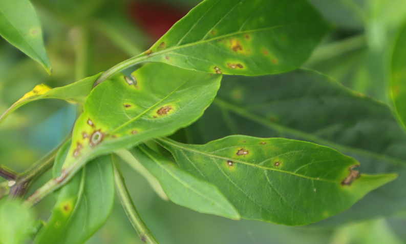
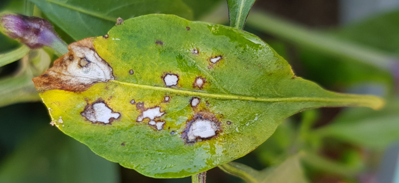
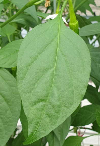
최근 Transformer 기반의 모델들이 각광을 받고 있다. 관련 코드를 보고, AI hub에 있는 데이터셋을 받아서 고추 잎 이미지의 분류를 실시해보았다.
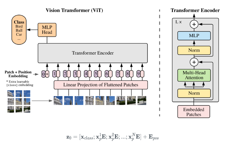
ViT Image classification 모델
https://keras.io/examples/vision/image_classification_with_vision_transformer/
Keras documentation: Image classification with Vision Transformer
Image classification with Vision Transformer Author: Khalid Salama Date created: 2021/01/18 Last modified: 2021/01/18 Description: Implementing the Vision Transformer (ViT) model for image classification. View in Colab • GitHub source Introduction This e
keras.io
AI Hub
AI-Hub
샘플 데이터 ? ※샘플데이터는 데이터의 이해를 돕기 위해 별도로 가공하여 제공하는 정보로써 원본 데이터와 차이가 있을 수 있으며, 데이터에 따라서 민감한 정보는 일부 마스킹(*) 처리가 되
www.aihub.or.kr
병든 잎사귀
정상 잎사귀

import numpy as np
import tensorflow as tf
from tensorflow import keras
from tensorflow.keras import layers
import tensorflow_addons as tfa
import cv2
import cvlib
import matplotlib.pyplot as plt
import numpy as np
import os
import pandas as pd
import seaborn as sns
from IPython.display import Image
from sklearn.metrics import confusion_matrix
from tensorflow.keras.preprocessing.image import array_to_img, load_img, img_to_array
from tensorflow.keras.layers import Conv2D, MaxPool2D, Dense, Flatten, Dropout
from tensorflow.keras.layers.experimental.preprocessing import RandomFlip, RandomRotation, RandomCrop
from tensorflow.keras.optimizers import Adam
from tensorflow.keras.models import Sequential
from tensorflow.keras.models import load_model
import PIL.Image
import PIL.ImageFilter
import io
import tensorflow_addons as tfa
Prepare the data
nomal_list = os.listdir('./nomal_leaf/')
nomal_list = [file for file in nomal_list if file.endswith(".jpg")]
diseaster_list = os.listdir('./dis_leaf/')
diseaster_list = [file for file in diseaster_list if file.endswith(".jpg")]
128 by 128 이미지 사이즈로 설정하여 실시함
image_height = 128
image_width = 128

images = []
labels = []

# 정상 0 질병 1
for nomal_row in nomal_list:
    image = load_img('./nomal_leaf/'+nomal_row, target_size=(image_height, image_width))
    image = img_to_array(image)
    images.append(image)
    labels.append(0)


# dis_label = np.array(dis_label)

for dis_row in diseaster_list:
    image = load_img('./dis_leaf/'+dis_row, target_size=(image_height, image_width))
    image = img_to_array(image)
    images.append(image)
    labels.append(1)
데이터 분리
from sklearn.model_selection import train_test_split
import numpy as np
input_shape = (128, 128, 3)
num_classes = 2
X = np.array(images) / 255. # 255 로 나누어주어 0~1 사이의 값으로 만들어줍니다.
y = np.array(labels)

x_train, x_test, y_train, y_test = train_test_split(X, y, test_size=0.4, shuffle = True, random_state = 0)
print(f"x_train shape: {x_train.shape} - y_train shape: {y_train.shape}")
print(f"x_test shape: {x_test.shape} - y_test shape: {y_test.shape}")
x_train shape: (50000, 32, 32, 3) - y_train shape: (50000, 1)
x_test shape: (10000, 32, 32, 3) - y_test shape: (10000, 1)
hyperparameters 설정
learning_rate = 0.001
weight_decay = 0.0001
batch_size = 16
num_epochs = 100
image_size = 32  # We'll resize input images to this size
patch_size = 6  # Size of the patches to be extract from the input images
num_patches = (image_size // patch_size) ** 2
projection_dim = 64
num_heads = 4
transformer_units = [
    projection_dim * 2,
    projection_dim,
]  # Size of the transformer layers
transformer_layers = 8
mlp_head_units = [2048, 1024]  # Size of the dense layers of the final classifier
데이터 증강
data_augmentation = keras.Sequential(
    [
        layers.Normalization(),
        layers.Resizing(image_size, image_size),
        layers.RandomFlip("horizontal"),
        layers.RandomRotation(factor=0.02),
        layers.RandomZoom(
            height_factor=0.2, width_factor=0.2
        ),
    ],
    name="data_augmentation",
)
# Compute the mean and the variance of the training data for normalization.
data_augmentation.layers[0].adapt(x_train)
멀티레이어 코드
def mlp(x, hidden_units, dropout_rate):
    for units in hidden_units:
        x = layers.Dense(units, activation=tf.nn.gelu)(x)
        x = layers.Dropout(dropout_rate)(x)
    return x
패치 생성 구현
class Patches(layers.Layer):
    def __init__(self, patch_size):
        super(Patches, self).__init__()
        self.patch_size = patch_size

    def call(self, images):
        batch_size = tf.shape(images)[0]
        patches = tf.image.extract_patches(
            images=images,
            sizes=[1, self.patch_size, self.patch_size, 1],
            strides=[1, self.patch_size, self.patch_size, 1],
            rates=[1, 1, 1, 1],
            padding="VALID",
        )
        patch_dims = patches.shape[-1]
        patches = tf.reshape(patches, [batch_size, -1, patch_dims])
        return patches
패치 인코딩 단계적 구현
PatchEncoder 레이어는 패치를 projection_dim 크기의 벡터로 투영하여 선형으로 패치를 변환합니다. 또한 투영된 벡터에 학습 가능한 위치 임베딩을 추가
class PatchEncoder(layers.Layer):
    def __init__(self, num_patches, projection_dim):
        super(PatchEncoder, self).__init__()
        self.num_patches = num_patches
        self.projection = layers.Dense(units=projection_dim)
        self.position_embedding = layers.Embedding(
            input_dim=num_patches, output_dim=projection_dim
        )

    def call(self, patch):
        positions = tf.range(start=0, limit=self.num_patches, delta=1)
        encoded = self.projection(patch) + self.position_embedding(positions)
        return encoded
ViT 모델 제작
ViT 모델은 여러 개의 Transformer 블록으로 구성되며, self-attention 메커니즘으로 'layers.MultiHeadAttention' 레이어를 사용하는 패치 시퀀스에 적용됨. 트랜스포머 블록은 [batch_size, num_patches, projection_dim] 텐서는 다음을 통해 처리
최종 클래스 확률 출력을 생성하기 위해 softmax가 있는 분류기 헤드를 사용
제공할 인코딩된 패치 시퀀스에 학습 가능한 임베딩을 추가함. 이미지 표현으로 최종 Transformer 블록의 모든 출력은 layers.Flatten()'으로 모양을 변경하고 이미지로 사용 분류기 헤드에 대한 표현을 입력. 'layers.GlobalAveragePooling1D' 레이어는 Transformer 블록의 출력을 집계하는 대신 사용 가능
특히 패치의 수와 투영 치수가 클 때 사용.
def create_vit_classifier():
    inputs = layers.Input(shape=input_shape)
    # Augment data.
    augmented = data_augmentation(inputs)
    # Create patches.
    patches = Patches(patch_size)(augmented)
    # Encode patches.
    encoded_patches = PatchEncoder(num_patches, projection_dim)(patches)

    # Create multiple layers of the Transformer block.
    for _ in range(transformer_layers):
        # Layer normalization 1.
        x1 = layers.LayerNormalization(epsilon=1e-6)(encoded_patches)
        # Create a multi-head attention layer.
        attention_output = layers.MultiHeadAttention(
            num_heads=num_heads, key_dim=projection_dim, dropout=0.1
        )(x1, x1)
        # Skip connection 1.
        x2 = layers.Add()([attention_output, encoded_patches])
        # Layer normalization 2.
        x3 = layers.LayerNormalization(epsilon=1e-6)(x2)
        # MLP.
        x3 = mlp(x3, hidden_units=transformer_units, dropout_rate=0.1)
        # Skip connection 2.
        encoded_patches = layers.Add()([x3, x2])

    # Create a [batch_size, projection_dim] tensor.
    representation = layers.LayerNormalization(epsilon=1e-6)(encoded_patches)
    representation = layers.Flatten()(representation)
    representation = layers.Dropout(0.5)(representation)
    # Add MLP.
    features = mlp(representation, hidden_units=mlp_head_units, dropout_rate=0.5)
    # Classify outputs.
    logits = layers.Dense(num_classes)(features)
    # Create the Keras model.
    model = keras.Model(inputs=inputs, outputs=logits)
    return model
컴파일, 학습, 평가
def run_experiment(model):
    optimizer = tfa.optimizers.AdamW(
        learning_rate=learning_rate, weight_decay=weight_decay
    )

    model.compile(
        optimizer=optimizer,
        loss=keras.losses.SparseCategoricalCrossentropy(from_logits=True),
        metrics=[
            keras.metrics.SparseCategoricalAccuracy(name="accuracy"),
,
        ],
    )
 )

    history = model.fit(
        x=x_train,
        y=y_train,
        batch_size=batch_size,
        epochs=num_epochs,
        validation_split=0.1,
    )


    return history


vit_classifier = create_vit_classifier()
history = run_experiment(vit_classifier)
모델 평가
accuracy = history.history['accuracy']
val_accuracy = history.history['val_accuracy']

loss=history.history['loss']
val_loss=history.history['val_loss']

epochs_range = range(num_epochs)

plt.figure(figsize=(16, 8))
plt.subplot(1, 2, 1)
plt.plot(epochs_range, accuracy, label='Training Accuracy')
plt.plot(epochs_range, val_accuracy, label='Validation Accuracy')
plt.legend(loc='lower right')
plt.title('Training and Validation Accuracy')

plt.subplot(1, 2, 2)
plt.plot(epochs_range, loss, label='Training Loss')
plt.plot(epochs_range, val_loss, label='Validation Loss')
plt.legend(loc='upper right')
plt.title('Training and Validation Loss')
plt.show()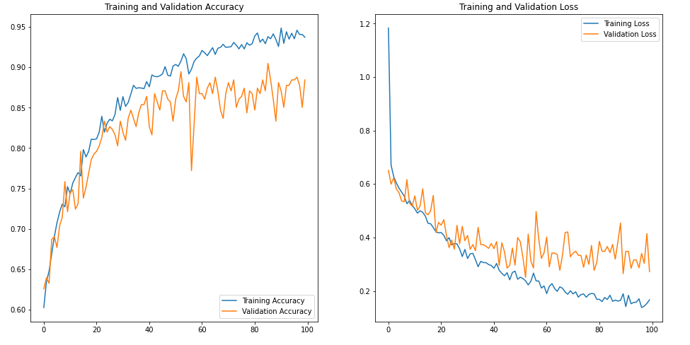
test_loss, test_accuracy = vit_classifier.evaluate(x_test, y_test, verbose=0)

print('test set accuracy: ', test_accuracy)
test set accuracy: 0.8834356069564819test_prediction = np.argmax(vit_classifier.predict(x_test), axis=-1)cm = confusion_matrix(y_test, test_prediction)
sns.heatmap(cm, annot = True)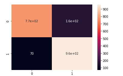
plt.figure(figsize = (13, 13))

start_index = 0
for i in range(len(y_test)):
    plt.subplot(5, 5, i + 1)
    plt.grid(False)
    plt.xticks([])
    plt.yticks([])
    prediction = test_prediction[start_index + i]
    actual = y_test[start_index + i]
    col = 'g'
    if prediction != actual:
        col = 'r'
    plt.xlabel('Actual={} || Pred={}'.format(actual, prediction), color = col)
    pimg = array_to_img(x_test[start_index + i, :, :, ::-1])
    plt.imshow(pimg)
plt.show()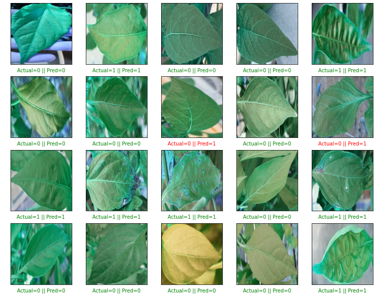
구글 검색에서 3개 이미지를 갖고와서 확인해봄
from PIL import Image
X = []

image_w = 128
image_h = 128
img = Image.open("sample.jpg")
img = img.convert("RGB")
# img.show()
img = img.resize((image_w, image_h))
data = np.asarray(img)
X.append(data)
X = np.array(X) / 255
X.shape
Y = []


img = Image.open("sample2.jpg")
img = img.convert("RGB")
# img.show()
img = img.resize((image_w, image_h))
data = np.asarray(img)
Y.append(data)
Y = np.array(Y) / 255
Y.shape

Z = []

img = Image.open("sample3.png")
img = img.convert("RGB")
img = img.resize((image_w, image_h))
# img.show()
data = np.asarray(img)
Z.append(data)
Z = np.array(Z) / 255
Z.shape


D = []

img = Image.open("sample4.png")
img = img.convert("RGB")
img = img.resize((image_w, image_h))
img.show()
data = np.asarray(img)
D.append(data)
D = np.array(D) / 255
D.shape
test_prediction_1 = np.argmax(vit_classifier.predict(X), axis=-1)
test_prediction_2 = np.argmax(vit_classifier.predict(Y), axis=-1)
test_prediction_3 = np.argmax(vit_classifier.predict(Z), axis=-1)
test_prediction_4 = np.argmax(vit_classifier.predict(D), axis=-1)
모델 튜닝, 데이터셋 증설 등으로 정확도를 좀 더 올리는게 가능해보인다.
'파이썬 이것저것 > 파이썬 딥러닝 관련' 카테고리의 다른 글
| [TensorRT] ValueError: cannot reshape array of size 57603 into shape (360,360) - ValueError 해결 (0) | 2022.10.30 |
|---|---|
| [python] Yolo v5 object detection 고추 병해 데이터 셋 학습해보기 (0) | 2022.08.02 |
| [Python] 딥러닝 ResNet 구현하기 (0) | 2022.07.17 |
| [Python] 딥러닝 CNN(VGG16 모델 구현하기) (0) | 2022.07.17 |
| [Python] 딥러닝 CNN 연산 (0) | 2022.07.17 |