반응형
https://www.tensorflow.org/tutorials/keras/classification?hl=ko
기본 분류: 의류 이미지 분류 | TensorFlow Core
기본 분류: 의류 이미지 분류 이 튜토리얼에서는 운동화나 셔츠 같은 옷 이미지를 분류하는 신경망 모델을 훈련합니다. 상세 내용을 모두 이해하지 못해도 괜찮습니다. 여기서는 완전한 텐서플
www.tensorflow.org
fashion_mnist = tf.keras.datasets.fashion_mnist
In [ ]:
import pandas as pd
import tensorflow as tf
import matplotlib.pyplot as plt
In [ ]:
fashion_mnist = tf.keras.datasets.fashion_mnist

(train_images, train_labels), (test_images, test_labels) = fashion_mnist.load_data()
In [ ]:
train_Y
Out[ ]:
array([9, 0, 0, ..., 3, 0, 5], dtype=uint8)In [ ]:
# 각 이미지 셋은 하난의 레이블에 매핑 됨
# 데이터셋 클래스 이름을 들어있지 않기 때문에
# 나중에 이미지를 출력할 때 사용하기 위해 별도의 변수를 만들어 저장
class_names = ['T-shirt/top', 'Trouser', 'Pullover', 'Dress', 'Coat',
               'Sandal', 'Shirt', 'Sneaker', 'Bag', 'Ankle boot']
class_name
Out[ ]:
['T-sharit',
 'Trouser',
 'Pullover',
 'Dress',
 'Coat',
 'Sandal',
 'Shirt',
 'Sneaker',
 'Bag',
 'Ankle boot']
In [ ]:
# 모델을 훈련하기 전에 데이터셋 구조를 파악
# 다음 코든느 훈련 세트에 60,000개의 이미지가 있따는 것을 보여줌
# 각 이미지는 28x28 픽셀오 표현된다.
train_images.shape
Out[ ]:
(60000, 28, 28)In [ ]:
len(train_labels)
Out[ ]:
60000In [ ]:
train_Y
Out[ ]:
array([9, 0, 0, ..., 3, 0, 5], dtype=uint8)In [ ]:
# 네트워크를 훈련하기 전에 데이터를 전처리 해야함
# 훈련 세트에 있는 첫 번째 이미지는
# 시각화를 통해 알 수 있다.
# 픽셀 값의 범위가 0~255 사이라는 것을 알 수 있다
plt.figure()
plt.imshow(train_images[0])
plt.colorbar()
plt.grid(False)
plt.show()

In [ ]:
train_images = train_images / 255.0

test_images = test_images / 255.0
In [ ]:
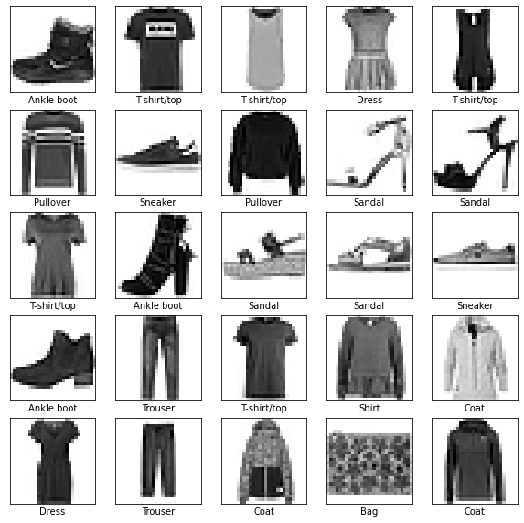
plt.figure(figsize=(10,10))
for i in range(25):
    plt.subplot(5,5,i+1)
    plt.xticks([])
    plt.yticks([])
    plt.grid(False)
    plt.imshow(train_images[i], cmap=plt.cm.binary)
    plt.xlabel(class_names[train_labels[i]])
plt.show()
In [ ]:
# 모델 구성
# 신경망의 기본 구성 요소는 층
# 층은 주입된 데이터에서 표현을 추출,
# 대부분 딥러닝은 간단한 층을 연결하여 구성
# tf.keras.lyaers.Dense 와 같은 층들의 가중치(paramter=w)는 훈련하는 동안 학습됨

model = tf.keras.Sequential([
                             tf.keras.layers.Flatten(input_shape=(28,28)),
                             tf.keras.layers.Dense(128, activation="relu"),
                             tf.keras.layers.Dense(10, activation="softmax")
])
In [ ]:
# 모델을 훈련하기 전에 필요한 몇 가지 설정이 모델 컴파일 단계에 추가
# 손실 함수 : 훈련하는 동안 모델의 오차를 측정, 모델의 학습이 올바른 방향으로 향하도록 이 함수를 최소화
# 옵티마이저 : 데이터와 손실 함수를 바탕으로 모델의 업데이트 방법을 결정
# 지표-훈련 단계와 테스트 단계를 모니터링하기 위해 사용
model.compile(optimizer='adam',
              loss=tf.keras.losses.SparseCategoricalCrossentropy(from_logits=True),
              metrics=['accuracy'])
In [ ]:
model.fit(train_images, train_labels, epochs=5)
Epoch 1/5
/usr/local/lib/python3.7/dist-packages/tensorflow/python/util/dispatch.py:1082: UserWarning: "`sparse_categorical_crossentropy` received `from_logits=True`, but the `output` argument was produced by a sigmoid or softmax activation and thus does not represent logits. Was this intended?"
  return dispatch_target(*args, **kwargs)
1875/1875 [==============================] - 5s 2ms/step - loss: 0.4971 - accuracy: 0.8255
Epoch 2/5
1875/1875 [==============================] - 4s 2ms/step - loss: 0.3777 - accuracy: 0.8650
Epoch 3/5
1875/1875 [==============================] - 4s 2ms/step - loss: 0.3413 - accuracy: 0.8753
Epoch 4/5
1875/1875 [==============================] - 4s 2ms/step - loss: 0.3150 - accuracy: 0.8842
Epoch 5/5
1875/1875 [==============================] - 4s 2ms/step - loss: 0.2966 - accuracy: 0.8908
Out[ ]:
<keras.callbacks.History at 0x7fb11beeec90>In [ ]:
# 정확도 평가
test_loss, test_acc = model.evaluate(test_images, test_labels, verbose=2)
print("테스트 정확도: ", test_acc)
313/313 - 0s - loss: 0.3447 - accuracy: 0.8771 - 375ms/epoch - 1ms/step
테스트 정확도:  0.8770999908447266
In [ ]:
# 훈련된 모델을 사용하여 이미지에 대한 예측을 만들 수 있다.
predictions = model.predict(test_images)
In [ ]:
# 첫 번째 예측을 확인
predictions[0]
Out[ ]:
array([2.9822331e-05, 7.0461623e-09, 1.7066720e-06, 1.9692172e-09,
       1.0831801e-06, 1.1030550e-02, 6.6612421e-07, 4.4927213e-02,
       1.5970636e-06, 9.4400734e-01], dtype=float32)
In [ ]:
import numpy as np
In [ ]:
# 10개 숫자 배열로 나타낸다
# 이 값은 10개의 옷 품목에 상응하는 모델의 신뢰도를 나타냄
# 가장 높은 신뢰도를 가진 레이블 검색
np.argmax(predictions[33])
Out[ ]:
2In [ ]:
test_labels[33]
Out[ ]:
3In [ ]:
def plot_image(i, predictions_array, true_label, img):
  true_label, img = true_label[i], img[i]
  plt.grid(False)
  plt.xticks([])
  plt.yticks([])

  plt.imshow(img, cmap=plt.cm.binary)

  predicted_label = np.argmax(predictions_array)
  if predicted_label == true_label:
    color = 'blue'
  else:
    color = 'red'

  plt.xlabel("{} {:2.0f}% ({})".format(class_names[predicted_label],
                                100*np.max(predictions_array),
                                class_names[true_label]),
                                color=color)

def plot_value_array(i, predictions_array, true_label):
  true_label = true_label[i]
  plt.grid(False)
  plt.xticks(range(10))
  plt.yticks([])
  thisplot = plt.bar(range(10), predictions_array, color="#777777")
  plt.ylim([0, 1])
  predicted_label = np.argmax(predictions_array)

  thisplot[predicted_label].set_color('red')
  thisplot[true_label].set_color('blue')
In [ ]:
i = 0
plt.figure(figsize=(6,3))
plt.subplot(1,2,1)
plot_image(i, predictions[i], test_labels, test_images)
plt.subplot(1,2,2)
plot_value_array(i, predictions[i],  test_labels)
plt.show()

In [ ]:
num_rows = 5
num_cols = 3
num_images = num_rows*num_cols
plt.figure(figsize=(2*2*num_cols, 2*num_rows))
for i in range(num_images):
  plt.subplot(num_rows, 2*num_cols, 2*i+1)
  plot_image(i, predictions[i], test_labels, test_images)
  plt.subplot(num_rows, 2*num_cols, 2*i+2)
  plot_value_array(i, predictions[i], test_labels)
plt.tight_layout()
plt.show()

'경기도 인공지능 개발 과정 > Python' 카테고리의 다른 글
| [Python] 텐서플로를 이용한 아이리스 분류 예측 (0) | 2022.07.11 |
|---|---|
| [Python] 텐서플로를 이용한 보스턴 집값 예측 (0) | 2022.07.11 |
| [Python] tkinter 를 이용한 데이터 분석 GUI 개발하기 (0) | 2022.07.10 |
| [Python] tkinter를 이용한 GUI 개발 (0) | 2022.07.10 |
| [파이썬 머신러닝] 회귀, 능형회귀, 로지스틱회귀 (0) | 2022.07.08 |