반응형
이미지 데이터의 이해
- 차원의 이해
- 차원 : 칼럼의 관점에서 각 데이터들은 2차원 평면에서 점으로 표현될 수 있다. 여기서 변수를 하나 더 추가한다면, 3차원 공간이 된다. 즉, 칼럼의 갯수가 n개라면, n차원의 공간의 한 점으로 표현이 가능하다.
- 이미지 데이터
- 이미지 데이터는 숫자들의 집합이 2차원 형태로 이루어져 있다. 예를 들어 (28,28)가로세로가 이루어져 있다면, 이 안에 숫자는 두개를 곱한 784개의 숫자가 존재한다.
- 이러한 이미지가 6만장 준비되어 있다면 (60000, 28, 28)의 형태가 되는것이다.
- 흑백이미지와 다르게, 컬러 이미지는 숫자 집합이 3개 존재한다. 각각 R(red) G(green) B(blue) 3가지로 구성되는 숫자들이다. 컬러는 각 칸에 숫자가 3개씩 들어 있다. 빨강과 녹색과 파랑에 대한 숫자가 컬러 이미지 내에 포함되어 있다.
MNIST 손글씨 실습
- MNIST의 6만장의 손글씨를 가져와 이를 출력해봄, 회색조 이미지
In [1]:
import tensorflow as tf
샘플 이미지셋 불러오기
In [15]:
(mnist_x, mnist_y), _ = tf.keras.datasets.mnist.load_data()
print(mnist_x.shape,mnist_y.shape)
(60000, 28, 28) (60000,)
In [6]:
import matplotlib.pyplot as plt
plt.imshow(mnist_x[0], cmap="gray")
Out[6]:
<matplotlib.image.AxesImage at 0x7f38d283c750>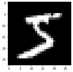
In [7]:
print(mnist_y[0])
5
In [8]:
print(mnist_y[0:10])
[5 0 4 1 9 2 1 3 1 4]
In [9]:
plt.imshow(mnist_x[1],cmap="gray")
Out[9]:
<matplotlib.image.AxesImage at 0x7f38d227ae50>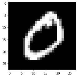
In [10]:
plt.imshow(mnist_x[2],cmap="gray")
Out[10]:
<matplotlib.image.AxesImage at 0x7f38d2214a10>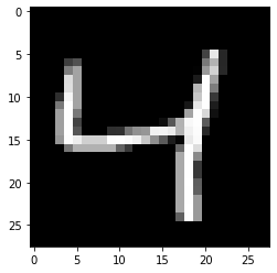
In [11]:
plt.imshow(mnist_x[4],cmap="gray")
Out[11]:
<matplotlib.image.AxesImage at 0x7f38d2181dd0>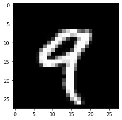
CIFAR-10 실습
- CIFAR-10 데이터를 출력해봄
In [19]:
(cifar_x, cifar_y), _ = tf.keras.datasets.cifar10.load_data()
print(cifar_x.shape, cifar_y.shape)
(50000, 32, 32, 3) (50000, 1)
In [21]:
print(cifar_x[0])
plt.imshow(cifar_x[0])
[[[ 59  62  63]
  [ 43  46  45]
  [ 50  48  43]
  ...
  [158 132 108]
  [152 125 102]
  [148 124 103]]

 [[ 16  20  20]
  [  0   0   0]
  [ 18   8   0]
  ...
  [123  88  55]
  [119  83  50]
  [122  87  57]]

 [[ 25  24  21]
  [ 16   7   0]
  [ 49  27   8]
  ...
  [118  84  50]
  [120  84  50]
  [109  73  42]]

 ...

 [[208 170  96]
  [201 153  34]
  [198 161  26]
  ...
  [160 133  70]
  [ 56  31   7]
  [ 53  34  20]]

 [[180 139  96]
  [173 123  42]
  [186 144  30]
  ...
  [184 148  94]
  [ 97  62  34]
  [ 83  53  34]]

 [[177 144 116]
  [168 129  94]
  [179 142  87]
  ...
  [216 184 140]
  [151 118  84]
  [123  92  72]]]
Out[21]:
<matplotlib.image.AxesImage at 0x7f38d216cbd0>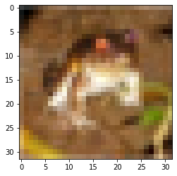
In [25]:
print(cifar_y[1])
plt.imshow(cifar_x[1])
[9]
Out[25]:
<matplotlib.image.AxesImage at 0x7f38d19a4510>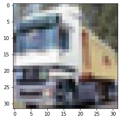
데이터 형태로 차원을 이해하는 방법
- 넘파이를 이용하여 데이터 형태를 나타내봄
In [26]:
import numpy as np
In [31]:
# 1차원
d1 = np.array([1,2,3,4,5])
print(d1.shape)
(5,)
In [32]:
# 2차원
d2 = np.array([d1, d1, d1, d1])
print(d2.shape)
(4, 5)
In [37]:
# 3차원
d3 = np.array([d2, d2, d2])
print(d3.shape)
(3, 4, 5)
In [38]:
# 4차원
d4 = np.array([d3, d3, d3])
print(d4.shape)
(3, 3, 4, 5)
MINST와 CIFAR-10의 종속변수의 형태를 비교하기
In [42]:
# shape가 다름을 알 수 있음
print(mnist_y.shape)
print(cifar_y.shape)
(60000,)
(50000, 1)
In [44]:
# 넘파이 형태로 나타내봄
x1 = np.array([1, 2, 3, 4, 5])
print(x1.shape)
(5,)
In [48]:
# mnist의 형태도 확인해봄
print(mnist_y[0:5])
print(mnist_y[0:5].shape)
[5 0 4 1 9]
(5,)
In [51]:
x2 = np.array([[1,2,3,4,5]])
print(x2.shape)
(1, 5)
In [54]:
x3 = np.array([[1],[2],[3],[4],[5]])
print(x3.shape)
print(cifar_y[0:5])
print(cifar_y[0:5].shape)
(5, 1)
[[6]
 [9]
 [9]
 [4]
 [1]]
(5, 1)'경기도 인공지능 개발 과정 > Python' 카테고리의 다른 글
| [Python] 텐서플로_컨볼루전(Conv2D)_실습 (0) | 2022.07.12 |
|---|---|
| [Python] 텐서플로 플래튼 (0) | 2022.07.12 |
| [Python] 텐서플로 히든레이어를 이용한 보스턴 집값과 아이리스 품종 예측 (0) | 2022.07.11 |
| [Python] 텐서플로를 이용한 아이리스 분류 예측 (0) | 2022.07.11 |
| [Python] 텐서플로를 이용한 보스턴 집값 예측 (0) | 2022.07.11 |