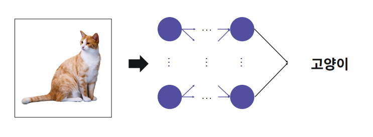
이미지 분류
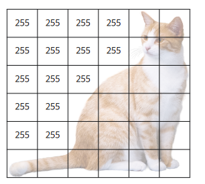
컴퓨터에게 이미지는 각 픽셀 값을 가진 숫자 배열로 인식
다양한 방법으로 이미지가 변형될 수 있는데 그러한 변화에도 강인한 이미지 처리를 어떻게 할 것인가
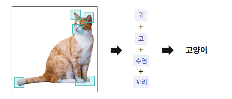
CNN 딥러닝 이전 컴퓨터 비전은 각 특징을 찾아서 특징을 중점으로 인식
이미지 데이터 확인해보기
Numpy, PIL, tensorflow.keras 등을 이용하여 이미지를 Numpy 배열로 바꿔보고, 이를 통해 이미지가 어떻게 이루어졌는지 확인
import  pandas as pd
import numpy as np

import PIL
import matplotlib.image as img
import matplotlib.pyplot as plt

from elice_utils import EliceUtils
elice_utils = EliceUtils()

# 이미지 목록을 불러오는 함수

def load_data(path):
    return pd.read_csv(path)

'''
1. PIL.Image를 이용하여
   이름(경로+이름)을 바탕으로 이미지를 불러오고,
   이를 리스트 'images'에 추가하는 함수를 완성
'''

def load_images(path, names):

    images=[]

    for name in names:
        images.append(PIL.Image.open(path + name))

    return images

'''
2. 이미지의 사이즈를 main 함수에 있는 'IMG_SIZE'로
   조정하고, 이를 Numpy 배열로 변환하는 함수를 완성
'''

def images2numpy(images, size):

    output = []

    for image in images:
        output.append(np.array(image.resize(size)))

    return output


# 이미지에 대한 정보를 나타내주는 함수

def sampleVisualize(np_images):

    fileName = "./data/images/1000092795.jpg"
    ndarray = img.imread(fileName)

    plt.imshow(ndarray)
    plt.show()
    plt.savefig("plot.png")

    print("\n1-1. 'fileName' 이미지(원본): ")
    elice_utils.send_image("plot.png")

    print('\n1-2. Numpy array로 변환된 원본 이미지:', ndarray)
    print('\n1-3. Numpy array로 변환된 원본 이미지의 크기:', np.array(ndarray).shape)

    plt.imshow(np_images[0])
    plt.show()
    plt.savefig("plot_re.png")

    print("\n2-1. 'fileName' 이미지(resize 후): ")
    elice_utils.send_image("plot_re.png")

    print('\n2-2. Numpy array로 변환된 resize 후 이미지:', np_images[0])
    print('\n2-3. Numpy array로 변환된 resize 후 이미지 크기:', np.array(np_images[0]).shape)

    print('\n3. Numpy array로 변환된 resize 후 이미지 10장의 크기:', np.array(np_images).shape)

'''
3. main 함수를 완성
'''

def main():

    CSV_PATH = "./data/data.csv"
    IMG_PATH = "./data/images/"
    IMG_SIZE = (300,300)
    MAX_LEN = 30
    BATCH_SIZE = 2

    name_caption = load_data(CSV_PATH)
    names = name_caption['file_name']

    images = load_images(IMG_PATH, names)
    np_images = images2numpy(images, IMG_SIZE)

    sampleVisualize(np_images)

    return images, np_images

if __name__=='__main__':
    main()
일반 다층 퍼셉트론 모델(MLP)로 이미지 데이터 분류하기
MNIST 데이터를 다층 퍼셉트론 모델(MLP)을 만들고 학습
import numpy as np
import tensorflow as tf
from tensorflow.keras.utils import to_categorical
from visual import *

import logging, os
logging.disable(logging.WARNING)
os.environ["TF_CPP_MIN_LOG_LEVEL"] = "3"

# 동일한 실행 결과 확인을 위한 코드
np.random.seed(123)
tf.random.set_seed(123)

'''
1. MNIST 데이테 셋을 전처리하는 'preprocess' 함수를 완성

'''

def preprocess():

    # MNIST 데이터 세트를 불러옵니다.
    mnist = tf.keras.datasets.mnist

    # MNIST 데이터 세트를 Train set과 Test set으로 나누어 줍니다.
    (train_images, train_labels), (test_images, test_labels) = mnist.load_data()

    train_images = train_images / 255
    test_images = test_images / 255

    train_labels = to_categorical(train_labels, 10)
    test_labels = to_categorical(test_labels, 10)

    return train_images, test_images, train_labels, test_labels

'''
2. 다층 퍼셉트론(MLP) 모델을 생성
'''
def MLP():

    model = tf.keras.Sequential()
    model.add(tf.keras.layers.Flatten(input_shape = (28, 28)))
    model.add(tf.keras.layers.Dense(128, activation = "relu"))
    model.add(tf.keras.layers.Dense(64, activation = "relu"))
    model.add(tf.keras.layers.Dense(10, activation = "softmax"))

    return model

'''
3. 모델을 불러온 후 학습시키고 테스트 데이터에 대해 평가

'''

def main():

    train_images, test_images, train_labels, test_labels = preprocess()

    model = MLP()

    model.compile(loss="categorical_crossentropy", optimizer = "adam",
    metrics = ["accuracy"])
    model.summary()

    history = model.fit(train_images, train_labels, epochs=20, validation_data = (test_images, test_labels), batch_size = 128, verbose=2)

    loss, test_acc = model.evaluate(test_images,test_labels, verbose=0)

    print('\nTest Loss : {:.4f} | Test Accuracy : {}'.format(loss, test_acc))
    print('예측한 Test Data 클래스 : ',model.predict_classes(test_images))

    Visulaize([('MLP', history)], 'loss')

    return history

if __name__ == "__main__":
    main()
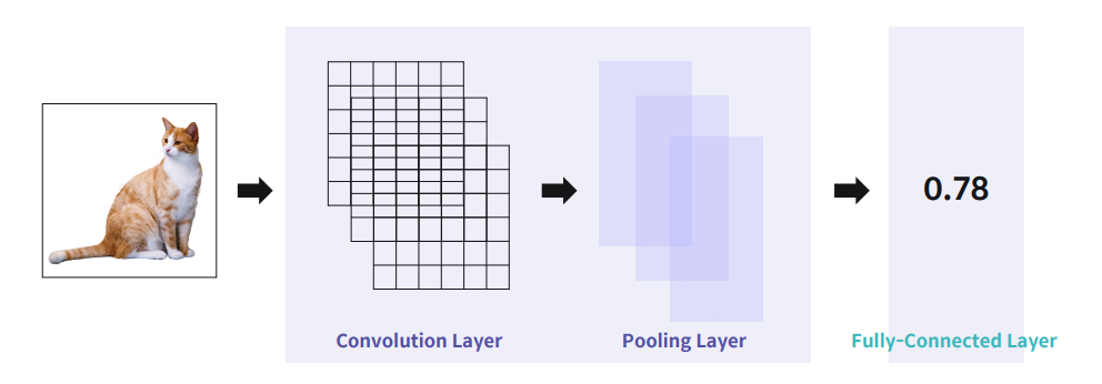
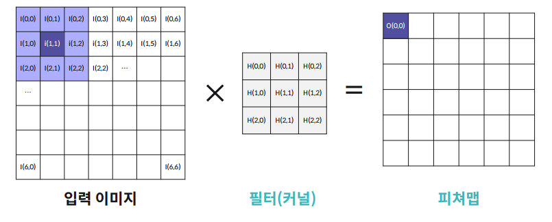
합성곱 신경망의 구조
눈코입 같은 패턴을 필터링 하여 pulling layer에서 작은 feature들을 줄이면서도 유의미한 패턴을 가지는
효과를 가지고 있음
입력이미지의 특징을 추출, 분류하는 과정으로 동작
Filter를 옆으로 한칸씩 넘어가면서 적용하여 특정한 값을 filter에 주고, input에 움직여가면서 곱해준다면
특정부분의 filter가 패턴이 있다고 판단하게 됨
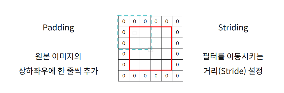
피쳐맵의 크기 변형 : Padding, Striding
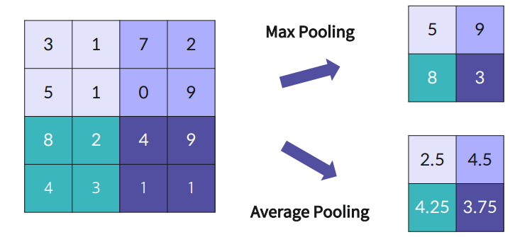
Pooling Layer
Pooling Layer는 2가지 Max Pooling과 Average Pooling 이 있다. 어떤 필터가 4 X 4 필터가 있다면
Pooling을 한다면 큰 이미지에서 필터를 옮겨가면서 적용을 하며 원하는 것을 찾으면서도 데이터가 너무 커지지 않게 해준다.
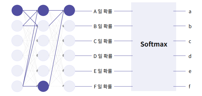
분류를 위한 Softmax 활성화 함수
고양이일 확률, 강아지, 자동차 등 확률값이 나오게 되는데, 가장 큰 값이 무엇일까를 보여주는게 Softmax 함수임
Convolution Layer 는 특징을 찾아내고, Pooling Layer 는 처리할 맵(이미지) 크기를 줄여준다. 이를 N 번 반복한다 반복할 때마다 줄어든 영역에서의 특징을 찾게 되고, 영역의 크기는 작아졌기 때문에 빠른 학습이 가능해진다.

Keras로 CNN 구현하기
일반적으로 CNN 모델은 Convolution 레이어 - MaxPooling 레이어 순서를 반복해 층을 쌓다가, 마지막 MaxPooling 레이어 다음에 Flatten 레이어를 하나 쌓고, 이후 몇 개의 Dense 레이어를 더 쌓아 완성
import numpy as np
import tensorflow as tf
from tensorflow.keras.utils import to_categorical
from visual import *
from plotter import *

import logging, os
logging.disable(logging.WARNING)
os.environ["TF_CPP_MIN_LOG_LEVEL"] = "3"

# 동일한 실행 결과 확인을 위한 코드
np.random.seed(123)
tf.random.set_seed(123)

'''
1. MNIST 데이테 셋을 전처리하는 'preprocess' 함수를 완성

'''

def preprocess():

    # MNIST 데이터 세트
    mnist = tf.keras.datasets.mnist

    # MNIST 데이터 세트를 Train set과 Test set으로 나누기
    (train_images, train_labels), (test_images, test_labels) = mnist.load_data()

    # Train 데이터 5000개와 Test 데이터 1000개를 사용
    train_images, train_labels = train_images[:5000], train_labels[:5000]
    test_images, test_labels = test_images[:1000], test_labels[:1000]

    train_images = train_images / 255
    test_images = test_images / 255

    train_images = np.expand_dims(train_images, -1)
    test_images = np.expand_dims(test_images, -1)

    train_labels = to_categorical(train_labels, 10)
    test_labels = to_categorical(test_labels, 10)

    return train_images, test_images, train_labels, test_labels

'''
2. CNN 모델을 생성
'''
def CNN():

    model = tf.keras.Sequential()
    model.add(tf.keras.layers.Conv2D(filters = 32, kernel_size = (3,3), activation = "relu", padding = "SAME", input_shape=(28, 28, 1)))
    model.add(tf.keras.layers.MaxPool2D(padding="SAME"))
    model.add(tf.keras.layers.Conv2D(filters = 32, kernel_size = (3,3), activation = "relu", padding = "SAME", input_shape=(28, 28, 1)))
    model.add(tf.keras.layers.MaxPool2D(padding="SAME"))
    model.add(tf.keras.layers.Conv2D(filters = 32, kernel_size = (3,3), activation = "relu", padding = "SAME", input_shape=(28, 28, 1)))
    model.add(tf.keras.layers.MaxPool2D(padding="SAME"))
    model.add(tf.keras.layers.Flatten())
    model.add(tf.keras.layers.Dense(64, activation= "relu"))
    model.add(tf.keras.layers.Dense(32, activation= "relu"))
    model.add(tf.keras.layers.Dense(10, activation= "softmax"))
    return model

'''
3. 모델을 불러온 후 학습시키고 테스트 데이터에 대해 평가

'''

def main():

    train_images, test_images, train_labels, test_labels = preprocess()

    model = CNN()

    model.summary()

    model.compile(loss= "categorical_crossentropy", optimizer = "adam", metrics=["accuracy"])

    history = model.fit(train_images, train_labels, epochs=15, batch_size=128,
    validation_data = (test_images, test_labels), verbose = 2)

    loss, test_acc = model.evaluate(test_images, test_labels, verbose=0)

    print('\nTest Loss : {:.4f} | Test Accuracy : {}'.format(loss, test_acc))
    print('예측한 Test Data 클래스 : ',model.predict_classes(test_images)[:10])

    Visulaize([('CNN', history)], 'loss')

    Plotter(test_images, model)

    return history

if __name__ == "__main__":
    main()
'파이썬 이것저것 > 파이썬 딥러닝 관련' 카테고리의 다른 글
| [Python] 딥러닝 순환 신경망 (RNN) (0) | 2022.07.15 |
|---|---|
| [Python] 딥러닝 자연어 처리를 위한 딥러닝 (0) | 2022.07.15 |
| [Python] 딥러닝 학습 속도 문제와 최적화-2 (0) | 2022.07.15 |
| [Python] 딥러닝 학습 속도 문제와 최적화 (0) | 2022.07.14 |
| [Python] 딥러닝 텐서플로 모델 구현하기 (0) | 2022.07.14 |