반응형
import numpy as np
import pandas as pd
import matplotlib.pyplot as plt
import sklearn.linear_model as lm
In [7]:
sap = pd.read_csv("sapXXI.csv").set_index("Date")
| 2200.169922 | 2277.530029 | 2187.439941 | 2238.830078 | 3710578000 | 2238.830078 |
| 2128.679932 | 2214.100098 | 2083.790039 | 2198.810059 | 4468273300 | 2198.810059 |
| 2164.330078 | 2169.600098 | 2114.719971 | 2126.149902 | 3672334700 | 2126.149902 |
| 2171.330078 | 2187.870117 | 2119.120117 | 2168.270020 | 3878265700 | 2168.270020 |
| 2173.149902 | 2193.810059 | 2147.580078 | 2170.949951 | 3451160800 | 2170.949951 |
| ... | ... | ... | ... | ... | ... |
| 1188.579956 | 1205.130005 | 1040.780029 | 1089.410034 | 6626699400 | 1089.410034 |
| 1171.229980 | 1219.800049 | 1170.689941 | 1186.689941 | 5847150900 | 1186.689941 |
| 1105.359985 | 1180.689941 | 1105.359985 | 1169.430054 | 4702951700 | 1169.430054 |
| 1073.890015 | 1112.420044 | 1044.500000 | 1104.489990 | 4658238400 | 1104.489990 |
| 1116.560059 | 1150.449951 | 1071.589966 | 1073.869995 | 5071601500 | 1073.869995 |
84 rows × 6 columns
In [10]:
sap.index = pd.to_datetime(sap.index)
sap_linear = sap.loc[sap.index > pd.to_datetime("2009-01-01")]
sap_linear
| 2200.169922 | 2277.530029 | 2187.439941 | 2238.830078 | 3710578000 | 2238.830078 |
| 2128.679932 | 2214.100098 | 2083.790039 | 2198.810059 | 4468273300 | 2198.810059 |
| 2164.330078 | 2169.600098 | 2114.719971 | 2126.149902 | 3672334700 | 2126.149902 |
| 2171.330078 | 2187.870117 | 2119.120117 | 2168.270020 | 3878265700 | 2168.270020 |
| 2173.149902 | 2193.810059 | 2147.580078 | 2170.949951 | 3451160800 | 2170.949951 |
| ... | ... | ... | ... | ... | ... |
| 1188.579956 | 1205.130005 | 1040.780029 | 1089.410034 | 6626699400 | 1089.410034 |
| 1171.229980 | 1219.800049 | 1170.689941 | 1186.689941 | 5847150900 | 1186.689941 |
| 1105.359985 | 1180.689941 | 1105.359985 | 1169.430054 | 4702951700 | 1169.430054 |
| 1073.890015 | 1112.420044 | 1044.500000 | 1104.489990 | 4658238400 | 1104.489990 |
| 1116.560059 | 1150.449951 | 1071.589966 | 1073.869995 | 5071601500 | 1073.869995 |
84 rows × 6 columns
In [14]:
# 모델을 준비하고 학습시킨다.
olm = lm.LinearRegression()
In [24]:
# sap_linear의 인덱스의 날짜를 누적일로 바꾼다.
# 1년 1월 1일부터 시작하여 누적된 날짜이다.
# 이를 numpy 배열로 바꾸고, 차원을 하나 높인다.
# 이 데이터는 X는 OLM회귀에서 독립 변수로 쓰인다

sap_linear = sap.loc[sap.index > pd.to_datetime("2009-01-01")]
X = np.array([x.toordinal() for x in sap_linear.index])[:, np.newaxis]
y = sap_linear["Close"]
In [25]:
# 학습 후, 예측을 수행한다.
# olm 모델을 적용하여 X를 이용하여 y를 적용해본다.
olm.fit(X, y)
Out[25]:
LinearRegression
LinearRegression()In [28]:
# 예측 수행
yp = [olm.predict([[x.toordinal()]])[0] for x in sap_linear.index]
In [30]:
# 모델을 평가한다.
olm_score = olm.score(X, y)
olm_score
Out[30]:
0.9395657944829205In [31]:
# 플로팅 스타일을 선택
# ggplot을 사용하여 시각화 작업
plt.style.use("ggplot")
In [35]:
# 두 데이터셋을 시각화한다,
# 실제 값과 예측 값에 각각 대응하는 그래프를 그린다
# LinearRegression 모델을 사용했으므로 예측값은 선형으로 출력

plt.plot(sap_linear.index, y)
plt.plot(sap_linear.index, yp)
plt.title("OLS Regression")
plt.xlabel("Year")
plt.ylabel("S&P 500(Closing)")
plt.legend(["Actual", "Predicted"], loc="lower right")
plt.annotate("Score=%.3f" % olm_score, xy=(pd.to_datetime("2010-06-01"), 1900))
Out[35]:
Text(2010-06-01 00:00:00, 1900, 'Score=0.940')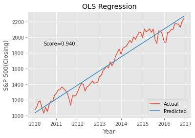
In [62]:
# 능형 회귀 Ridge Regression
# 두 개 이상의 예측 변수가 서로 강한 상관관계를 갖고 있는 것을 공선성 collinearity 라고 한다.
# 공선성은 OLM에 큰 오류를 가져온다
# 능형회귀는 이 문제를 해결하기 위해 고안된 선형 회귀 모델
# 알파를 사용하여 계수가 아상한 값을 갖지 않도록 제약한다
# 이률 정규화 regularziation라고 한다

# Ridge Regression 모델을 regr이라는 이름의 변수에 저장
# 알파를 미리 정의

regr = lm.Ridge(alpha=0.5)
regr.fit(X,y)
Out[62]:
Ridge
Ridge(alpha=0.5)In [63]:
# 예측 수행
yp = [regr.predict([[x.toordinal()]])[0] for x in sap_linear.index]
In [64]:
# 모델을 평가한다.
regr_score = regr.score(X, y)
regr_score
Out[64]:
0.9395657944829177In [66]:
# 두 데이터셋을 시각화한다,
# 실제 값과 예측 값에 각각 대응하는 그래프를 그린다
# LinearRegression 모델을 사용했으므로 예측값은 선형으로 출력

plt.plot(sap_linear.index, y)
plt.plot(sap_linear.index, yp)
plt.title("Ridge Regression")
plt.xlabel("Year")
plt.ylabel("S&P 500(Closing)")
plt.legend(["Actual", "Predicted"], loc="lower right")
plt.annotate("Score=%.3f" % olm_score, xy=(pd.to_datetime("2010-06-01"), 1900))
Out[66]:
Text(2010-06-01 00:00:00, 1900, 'Score=0.940')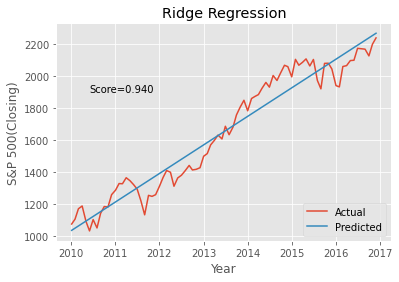
In [68]:
# 로지스틱 회귀
import pandas as pd
from sklearn.metrics import confusion_matrix
import sklearn.linear_model as lm
In [69]:
clf = lm.LogisticRegression(C=10.0)
In [78]:
grades = pd.read_table("grades.csv")
labels = ("F", "D", "C", "B", "A")
grades["Letter"] = pd.cut(grades["Final score"], [0, 60, 70, 80, 90, 100], labels=labels)
X = grades[["Quiz 1", "Quiz 2"]]

clf.fit(X, grades["Letter"])
Score = 0.558
c:\Users\Admin\AppData\Local\Programs\Python\Python39\lib\site-packages\sklearn\linear_model\_logistic.py:444: ConvergenceWarning: lbfgs failed to converge (status=1):
STOP: TOTAL NO. of ITERATIONS REACHED LIMIT.

Increase the number of iterations (max_iter) or scale the data as shown in:
    https://scikit-learn.org/stable/modules/preprocessing.html
Please also refer to the documentation for alternative solver options:
    https://scikit-learn.org/stable/modules/linear_model.html#logistic-regression
  n_iter_i = _check_optimize_result(
In [80]:
print("Score = %.3f" % clf.score(X, grades["Letter"]))
Score = 0.558
55%정도의 정확도가 나왔다. 2개 컬럼 치곤 높은 정확도인거 같다.
In [81]:
cm = confusion_matrix(clf.predict(X), grades["Letter"])
print(pd.DataFrame(cm, columns = labels, index=labels))
혼동행렬을 출력한다.
   F   D  C  B  A
F  0   0  0  0  0
D  2  15  4  3  1
C  0   2  7  2  1
B  0   0  1  0  1
A  0   0  0  2  2
In [85]:
import pickle, pandas as pd
In [92]:
alco2009 = pickle.load(open("alco2009.pickle", "rb"))
states = pd.read_csv("states.csv", names=("State", ""))
In [96]:
from sklearn.ensemble import RandomForestRegressor
import pandas as pd, numpy.random as rnd
import matplotlib.pyplot as plt
import matplotlib
In [107]:
hed
Out[107]:
crimzninduschasnoxrmagedisradtaxptratioblstatmedv01234...500501502503504
| 0.00632 | 18.0 | 2.31 | 0.0 | 0.538 | 6.575 | 65.2 | 4.0900 | 1.0 | 296.0 | 15.3 | 396.90 | 4.98 | 24.0 |
| 0.02731 | 0.0 | 7.07 | 0.0 | 0.469 | 6.421 | 78.9 | 4.9671 | 2.0 | 242.0 | 17.8 | 396.90 | 9.14 | 21.6 |
| 0.02729 | 0.0 | 7.07 | 0.0 | 0.469 | 7.185 | 61.1 | 4.9671 | 2.0 | 242.0 | 17.8 | 392.83 | 4.03 | 34.7 |
| 0.03237 | 0.0 | 2.18 | 0.0 | 0.458 | 6.998 | 45.8 | 6.0622 | 3.0 | 222.0 | 18.7 | 394.63 | 2.94 | 33.4 |
| 0.06905 | 0.0 | 2.18 | 0.0 | 0.458 | 7.147 | 54.2 | 6.0622 | 3.0 | 222.0 | 18.7 | 396.90 | 5.33 | 36.2 |
| ... | ... | ... | ... | ... | ... | ... | ... | ... | ... | ... | ... | ... | ... |
| 0.06263 | 0.0 | 11.93 | 0.0 | 0.573 | 6.593 | 69.1 | 2.4786 | 1.0 | 273.0 | 21.0 | 391.99 | 9.67 | 22.4 |
| 0.04527 | 0.0 | 11.93 | 0.0 | 0.573 | 6.120 | 76.7 | 2.2875 | 1.0 | 273.0 | 21.0 | 396.90 | 9.08 | 20.6 |
| 0.06076 | 0.0 | 11.93 | 0.0 | 0.573 | 6.976 | 91.0 | 2.1675 | 1.0 | 273.0 | 21.0 | 396.90 | 5.64 | 23.9 |
| 0.10959 | 0.0 | 11.93 | 0.0 | 0.573 | 6.794 | 89.3 | 2.3889 | 1.0 | 273.0 | 21.0 | 393.45 | 6.48 | 22.0 |
| 0.04741 | 0.0 | 11.93 | 0.0 | 0.573 | 6.030 | 80.8 | 2.5050 | 1.0 | 273.0 | 21.0 | 396.90 | 7.88 | 11.9 |
505 rows × 14 columns
In [109]:
### 데이터를 읽어들이고, 데이터셋을 2가지로 무작위 분리한다.###
# 부동산 가격에 영향을 주는 변수로 구성된 데이터 프레임이다.
# binomial() : 이산확률분포 따르는 데이터 값
# 이산 확률 분포 : 연속된 값이 아닌, 별개 값에 대한 확률을 부여하며 별개의 값이 나올 확률
# 예: 동전을 100번 던져서 앞, 뒤가 나오는 것을 기록함
hed = pd.read_csv("Hedonic.csv")
selection = rnd.binomial(1, 0.7, size=len(hed)).astype(bool)
training = hed[selection]
tseting = hed[~selection]
In [110]:
training.head()
Out[110]:
crimzninduschasnoxrmagedisradtaxptratioblstatmedv01234
| 0.00632 | 18.0 | 2.31 | 0.0 | 0.538 | 6.575 | 65.2 | 4.0900 | 1.0 | 296.0 | 15.3 | 396.90 | 4.98 | 24.0 |
| 0.02731 | 0.0 | 7.07 | 0.0 | 0.469 | 6.421 | 78.9 | 4.9671 | 2.0 | 242.0 | 17.8 | 396.90 | 9.14 | 21.6 |
| 0.02729 | 0.0 | 7.07 | 0.0 | 0.469 | 7.185 | 61.1 | 4.9671 | 2.0 | 242.0 | 17.8 | 392.83 | 4.03 | 34.7 |
| 0.03237 | 0.0 | 2.18 | 0.0 | 0.458 | 6.998 | 45.8 | 6.0622 | 3.0 | 222.0 | 18.7 | 394.63 | 2.94 | 33.4 |
| 0.06905 | 0.0 | 2.18 | 0.0 | 0.458 | 7.147 | 54.2 | 6.0622 | 3.0 | 222.0 | 18.7 | 396.90 | 5.33 | 36.2 |
In [111]:
tseting.head()
Out[111]:
crimzninduschasnoxrmagedisradtaxptratioblstatmedv6791012
| 0.08829 | 12.5 | 7.87 | 0.0 | 0.524 | 6.012 | 66.6 | 5.5605 | 5.0 | 311.0 | 15.2 | 395.60 | 12.43 | 22.9 |
| 0.14455 | 12.5 | 7.87 | 0.0 | 0.524 | 6.172 | 96.1 | 5.9505 | 5.0 | 311.0 | 15.2 | 396.90 | 19.15 | 27.1 |
| 0.17004 | 12.5 | 7.87 | 0.0 | 0.524 | 6.004 | 85.9 | 6.5921 | 5.0 | 311.0 | 15.2 | 386.71 | 17.10 | 18.9 |
| 0.22489 | 12.5 | 7.87 | 0.0 | 0.524 | 6.377 | 94.3 | 6.3467 | 5.0 | 311.0 | 15.2 | 392.52 | 20.45 | 15.0 |
| 0.09378 | 12.5 | 7.87 | 0.0 | 0.524 | 5.889 | 39.0 | 5.4509 | 5.0 | 311.0 | 15.2 | 390.50 | 15.71 | 21.7 |
In [114]:
rfr = RandomForestRegressor()
rfr
Out[114]:
RandomForestRegressor
RandomForestRegressor()In [116]:
prdictors_tra = training.loc[:, "crim":"lstat"]
prdictors_tst = tseting.loc[:, "crim":"lstat"]
In [118]:
feature = "medv"
rfr.fit(prdictors_tra, training[feature])
Out[118]:
RandomForestRegressor
RandomForestRegressor()In [128]:
plt.scatter(training[feature], rfr.predict(prdictors_tra), c= "green", s=50)
Out[128]:
<matplotlib.collections.PathCollection at 0x24b0a5b0280>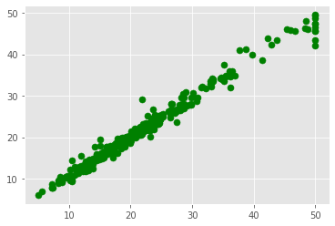
In [136]:
matplotlib.style.use("ggplot")
In [137]:
plt.scatter(training[feature], rfr.predict(prdictors_tra), c= "green", s=50)
plt.scatter(tseting[feature], rfr.predict(prdictors_tst), c="red")
Out[137]:
<matplotlib.collections.PathCollection at 0x24b0a79ff40>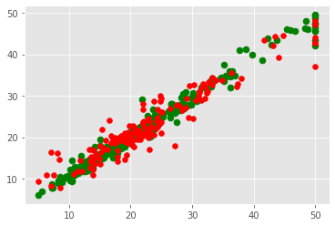
'경기도 인공지능 개발 과정 > Python' 카테고리의 다른 글
| [Python] tkinter 를 이용한 데이터 분석 GUI 개발하기 (0) | 2022.07.10 |
|---|---|
| [Python] tkinter를 이용한 GUI 개발 (0) | 2022.07.10 |
| [Python 데이터분석] 데이터 분석 기초 1 (0) | 2022.06.30 |
| [Python 데이터분석] matplotlib을 이용한 기본 시각화 (0) | 2022.06.30 |
| [django] TODOLIST 앱 등록해보기 (0) | 2022.06.10 |