데이터가 조금 더 복잡하다면?
각 매체가 얼마나 효율적인지 알아내 보자
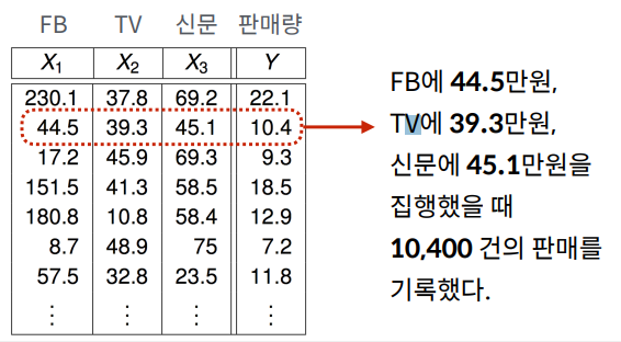
FB에 30만원, TV에 100만원, 신문에 50만원의 광고비를 집행했을 때 예상 판매량은 얼마인가?

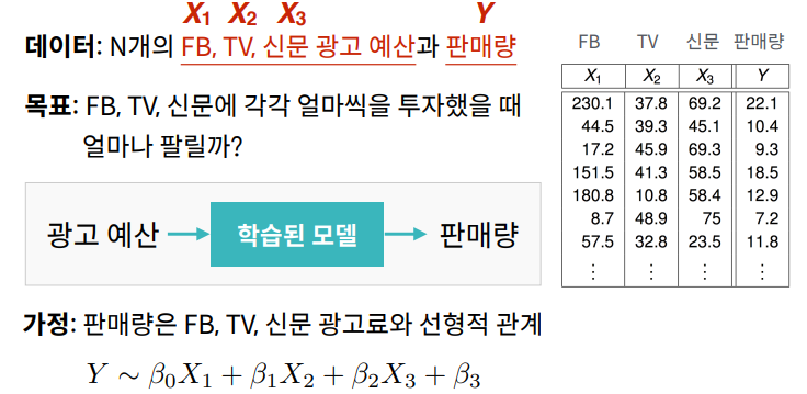
N: 데이터의 개수 FB TV 신문 판매량
X: “Input” 데이터/Feature (광고료)
- X1: FB 광고료
- X2: TV 광고료
- X3: 신문 광고료
Y: “Output” 해답/응답 (판매량)
(x1(i), x2(i), x3(i), y(i)): i번째 데이터
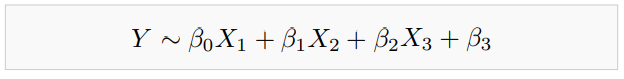
단순선형회귀분석과 동일 완벽한 예측은 불가능
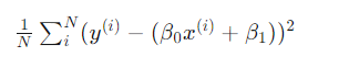
각 데이터 (x1(i), x2(i), x3(i), y(i)) 의 실제 값과 모델이 예측하는 값을 최소한으로 만들어줌
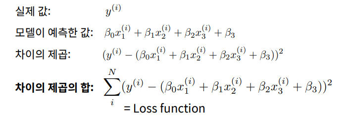
이 차이를 최소로 하는 β0, β1, β2, β3 을 구하도록 함
다중 회귀 분석
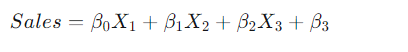
다중 회귀 분석(Multiple Linear Regression)은 데이터의 여러 변수(features) XX를 이용해 결과 YY를 예측하는 모델
import numpy as np
from sklearn.linear_model import LinearRegression
from sklearn.metrics import r2_score

'''
./data/Advertising.csv 에서 데이터를 읽어, X와 Y를 만듬

X는 (200, 3) 의 shape을 가진 2차원 np.array,
Y는 (200,) 의 shape을 가진 1차원 np.array여야 함

X는 FB, TV, Newspaper column 에 해당하는 데이터를 저장
Y는 Sales column 에 해당하는 데이터를 저장
'''

import csv
csvreader = csv.reader(open("data/Advertising.csv"))

x = []
y = []


next(csvreader)
for line in csvreader :
    x_i = [ float(line[1]), float(line[2]), float(line[3]) ]
    y_i = float(line[4])
    x.append(x_i)
    y.append(y_i)

X = np.array(x)
Y = np.array(y)

print(X)
print(Y)

lrmodel = LinearRegression()
lrmodel.fit(X, Y)

beta_0 = lrmodel.coef_[0] # 0번째 변수에 대한 계수 (페이스북)
beta_1 = lrmodel.coef_[1] # 1번째 변수에 대한 계수 (TV)
beta_2 = lrmodel.coef_[2] # 2번째 변수에 대한 계수 (신문)
beta_3 = lrmodel.intercept_ # y절편 (기본 판매량)

print("beta_0: %f" % beta_0)
print("beta_1: %f" % beta_1)
print("beta_2: %f" % beta_2)
print("beta_3: %f" % beta_3)

def expected_sales(fb, tv, newspaper, beta_0, beta_1, beta_2, beta_3):
    '''
    FB에 fb만큼, TV에 tv만큼, Newspaper에 newspaper 만큼의 광고비를 사용했고,
    트레이닝된 모델의 weight 들이 beta_0, beta_1, beta_2, beta_3 일 때
    예상되는 Sales 의 양을 출력
    '''

    sales = beta_0 * fb + beta_1 * tv + beta_2 * newspaper + beta_3

    return sales

print("예상 판매량: %f" % expected_sales(12, 10, 100, beta_0, beta_1, beta_2, beta_3))
다항회귀분석
단순한 선형회귀법은 데이터를 잘 설명하지 못한다. 조금 더 데이터에 맞게 모델을 학습시킬 수 없을까?
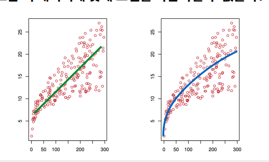
문제: 판매량과 광고비의 관계를 2차식으로 표현
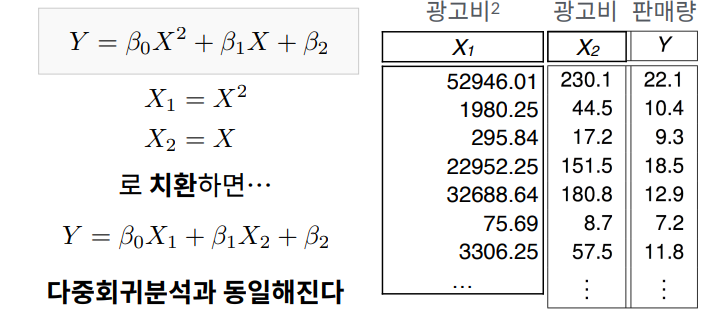
다항식 회귀 분석
다항식 회귀 분석(Polynomial Linear Regression)은 다중 선형 회귀 분석과 원리가 같습니다. 다만 데이터에 전처리를 함으로써 새로운 변수 간의 조합을 만들어낸 뒤 회귀 분석을 진행하는 것이 차이임
MSE란 평균제곱오차를 의미하며, 통계적 추정에 대한 정확성의 지표로 널리 이용됨
교차 검증
교차 검증이란 모델이 결과를 잘 예측하는지 알아보기 위해 전체 데이터를 트레이닝(training) 세트와 테스트(Test) 세트로 나누어 모델에 넣고 성능을 평가하는 방법
import numpy as np
from sklearn.linear_model import LinearRegression
from sklearn.metrics import mean_squared_error
from sklearn.model_selection import train_test_split

'''
./data/Advertising.csv 에서 데이터를 읽어, X와 Y를 만듬

X는 (200, 3) 의 shape을 가진 2차원 np.array,
Y는 (200,) 의 shape을 가진 1차원 np.array여야 함

X는 FB, TV, Newspaper column 에 해당하는 데이터를 저장
Y는 Sales column 에 해당하는 데이터를 저장
'''
import csv
csvreader = csv.reader(open("data/Advertising.csv"))
X = []
Y = []
next(csvreader)
for i in csvreader:
    x_i = [float(i[1]), float(i[2]), float(i[3])]
    X.append(x_i)
    y_i = [float(i[4])]
    Y.append(y_i)
print(X)
print(Y)
# 다항식 회귀분석을 진행하기 위해 변수들을 조합
X_poly = []
for x_i in X:
    X_poly.append([
        x_i[0] ** 2, # X_1^2
        x_i[1], # X_2
        x_i[1] * x_i[2], # X_2 * X_3
        x_i[1] ** 2,
        x_i[2] ** 2,
        x_i[2] + x_i[1],
        x_i[2] - x_i[1],
        x_i[2] * x_i[1],
        x_i[0] + x_i[2],
        x_i[2] / x_i[0],
        x_i[0] - x_i[2],
        x_i[0] * 3,
        x_i[1] * 1.2,


         # X_3
    ])

# X, Y를 80:20으로 나누기 80%는 트레이닝 데이터, 20%는 테스트 데이터
x_train, x_test, y_train, y_test = train_test_split(X_poly, Y, test_size=0.4, random_state=0)

# x_train, y_train에 대해 다항식 회귀분석을 진행
lrmodel = LinearRegression()
lrmodel.fit(x_train, y_train)

#x_train에 대해, 만든 회귀모델의 예측값을 구하고, 이 값과 y_train 의 차이를 이용해 MSE를 구하기
predicted_y_train = lrmodel.predict(x_train)
mse_train = mean_squared_error(y_train, predicted_y_train)
print("MSE on train data: {}".format(mse_train))

# x_test에 대해, 만든 회귀모델의 예측값을 구하고, 이 값과 y_test 의 차이를 이용해 MSE를 구 이 값이 1 미만이 되도록 모델을 구성
predicted_y_test = lrmodel.predict(x_test)
mse_test = mean_squared_error(y_test, predicted_y_test)
print("MSE on test data: {}".format(mse_test))
영어 단어 코퍼스 분석하기
British National Corpus (BNC) 텍스트 코퍼스(단어모음)를 활용하여
단어 10,000개의 빈도수를 그래프로 시각화한 후 선형회귀법을 적용
import operator
from sklearn.linear_model import LinearRegression
import numpy as np
import matplotlib
matplotlib.use('Agg')
import matplotlib.pyplot as plt
import elice_utils


def main():
    words = read_data()
    words = sorted(____________) # words.txt 단어를 빈도수 순으로 정렬

    # 정수로 표현된 단어를 X축 리스트에, 각 단어의 빈도수를 Y축 리스트에 저장
    X = list(range(1, len(words)+1))
    Y = [x[1] for x in words]

    # X, Y 리스트를 array로 변환
    X, Y = np.array(X).reshape(-1,1), np.array(Y)

    # X, Y의 각 원소 값에 log()를 적용
    # X, Y = np.log(X), np.log(Y)

    # 기울기와 절편을 구한 후 그래프와 차트를 출력
    slope, intercept = do_linear_regression(X, Y)
    draw_chart(X, Y, slope, intercept)

    return slope, intercept


# read_data() - words.txt에 저장된 단어와 해당 단어의 빈도수를 리스트형으로 변환
def read_data():
    # words.txt 에서 단어들를 읽어,
    # [[단어1, 빈도수], [단어2, 빈도수] ... ]형으로 변환해 리턴
    words = []

    return words


# do_linear_regression() - 임포트한 sklearn 패키지의 함수를 이용해 그래프의 기울기와 절편을 구함
def do_linear_regression(X, Y):
    # do_linear_regression() 함수를 작성

    return (slope, intercept)


# draw_chart() - matplotlib을 이용해 차트를 설정
def draw_chart(X, Y, slope, intercept):
    fig = plt.figure()
    ax = fig.add_subplot(111)
    plt.scatter(X, Y)

    # 차트의 X, Y축 범위와 그래프를 설정
    min_X = min(X)
    max_X = max(X)
    min_Y = min_X * slope + intercept
    max_Y = max_X * slope + intercept
    plt.plot([min_X, max_X], [min_Y, max_Y],
             color='red',
             linestyle='--',
             linewidth=3.0)

    # 기울과와 절편을 이용해 그래프를 차트에 입력
    ax.text(min_X, min_Y + 0.1, r'$y = %.2lfx + %.2lf$' % (slope, intercept), fontsize=15)

    plt.savefig('chart.png')
    elice_utils.send_image('chart.png')

if __name__ == "__main__":
main()'파이썬 이것저것 > 파이썬 머신러닝' 카테고리의 다른 글
| [Python] 머신러닝 K-means 클러스터링, PCA(차원축소) (0) | 2022.07.23 |
|---|---|
| [Python] 머신러닝 단순선형회귀분석 (0) | 2022.07.18 |
| [파이썬] XGB 활용하여 성적예측 (0) | 2022.04.23 |