반응형
Chapter 1. DataFrame 살펴보기
1. DataFrame이 뭔가요?
- DataFrame은 2차원(col과 row을 가짐)테이블 데이터 구조를 가지는 자료형
- Data Analysis, Machine Learning에서 data 변형을 위해 가장 많이 사용
- 주의 : Series나 DataFrame은 대소문자가 구분되므로 Series, DataFrame으로 사용
In [1]:
# pandas import
import pandas as pd
1-1. DataFrame 만들어 보기
Dictionary 형으로 생성
In [2]:
a1 = pd.DataFrame({"a" : [1,2,3], "b" : [4,5,6], "c" : [7,8,9]})
a1
Out[2]:
abc012
| 1 | 4 | 7 |
| 2 | 5 | 8 |
| 3 | 6 | 9 |
List 형태로 데이터 프레임 생성
In [3]:
# shift+tab을 활용
a2 = pd.DataFrame([[1,2,3], [4,5,6], [7,8,9]], ["a","b","c"])
a2
Out[3]:
012abc
| 1 | 2 | 3 |
| 4 | 5 | 6 |
| 7 | 8 | 9 |
1-2. 파일을 읽어서 DataFrame생성하기
- pandas.read_csv 함수 사용
- 대부분의 업무에서는 분석하고자 하는 Datat가 존재할 것
- 이를 읽어 들이는 것부터 데이터 분석의 시작!
- 이번 실습에서 읽을 파일 : data.csv
In [10]:
# kt 데이터 파일을 활용
cust = pd.read_csv('data.csv')
cust
Out[10]:
base_ymdpro_tgt_perd_valcust_ctg_typecust_classsex_typeageefct_svc_countdt_stop_ynnpay_ynr3m_avg_bill_amtr3m_A_avg_arpu_amtr3m_B_avg_arpu_amtr6m_A_avg_arpu_amtr6m_B_avg_arpu_amttermination_yn01234...99259926992799289929
| 202006 | 20200630 | 10001 | C | F | 28 | 0 | N | N | 2640.0000 | 792.000000 | 1584.0000 | 0.0 | 0.0000 | Y |
| 202006 | 20200630 | 10001 | _ | _ | _ | 1 | N | N | 300.0000 | 90.000000 | 180.0000 | 0.0 | 0.0000 | Y |
| 202006 | 20200630 | 10001 | E | F | 24 | 1 | N | N | 16840.0000 | 2526.000000 | 6983.0000 | 0.0 | 6981.0000 | N |
| 202006 | 20200630 | 10001 | F | F | 32 | 1 | N | N | 15544.7334 | 2331.710010 | 6750.4666 | 0.0 | 6508.8000 | N |
| 202006 | 20200630 | 10001 | D | M | 18 | 1 | N | N | 4700.0000 | 0.000000 | 4502.0000 | 0.0 | 4507.7000 | N |
| ... | ... | ... | ... | ... | ... | ... | ... | ... | ... | ... | ... | ... | ... | ... |
| 202006 | 20200630 | 10001 | C | F | 15 | 1 | N | Y | 1296.0999 | 194.414985 | 643.1001 | 0.0 | 852.5499 | N |
| 202006 | 20200630 | 10001 | G | M | 12 | 1 | N | N | 13799.6666 | 2069.949990 | 10605.9266 | 0.0 | 10603.9266 | N |
| 202006 | 20200630 | 10005 | C | _ | _ | 1 | N | N | 1396.2000 | 1206.000000 | 0.0000 | 1212.0 | 0.0000 | N |
| 202006 | 20200630 | 10001 | C | F | 40 | 0 | N | N | 3140.0000 | 942.000000 | 1884.0000 | 0.0 | 0.0000 | Y |
| 202006 | 20200630 | 10001 | C | F | 59 | 1 | N | N | 2436.9000 | 365.535000 | 1839.9000 | 0.0 | 1919.7999 | N |
9930 rows × 15 columns
- DataFrame 데이터 살펴보기DataFrame의 구조 (인덱스와 컬럼)
- 인덱스(Index) : 행의 레이블에 대한 정보를 보유하고 있음
- 컬럼(Columns) : 열의 레이블에 대한 정보를 보유하고 있음
- 인덱스와 컬럼 자체는 중복값일 수 없음
In [11]:
cust
Out[11]:
base_ymdpro_tgt_perd_valcust_ctg_typecust_classsex_typeageefct_svc_countdt_stop_ynnpay_ynr3m_avg_bill_amtr3m_A_avg_arpu_amtr3m_B_avg_arpu_amtr6m_A_avg_arpu_amtr6m_B_avg_arpu_amttermination_yn01234...99259926992799289929
| 202006 | 20200630 | 10001 | C | F | 28 | 0 | N | N | 2640.0000 | 792.000000 | 1584.0000 | 0.0 | 0.0000 | Y |
| 202006 | 20200630 | 10001 | _ | _ | _ | 1 | N | N | 300.0000 | 90.000000 | 180.0000 | 0.0 | 0.0000 | Y |
| 202006 | 20200630 | 10001 | E | F | 24 | 1 | N | N | 16840.0000 | 2526.000000 | 6983.0000 | 0.0 | 6981.0000 | N |
| 202006 | 20200630 | 10001 | F | F | 32 | 1 | N | N | 15544.7334 | 2331.710010 | 6750.4666 | 0.0 | 6508.8000 | N |
| 202006 | 20200630 | 10001 | D | M | 18 | 1 | N | N | 4700.0000 | 0.000000 | 4502.0000 | 0.0 | 4507.7000 | N |
| ... | ... | ... | ... | ... | ... | ... | ... | ... | ... | ... | ... | ... | ... | ... |
| 202006 | 20200630 | 10001 | C | F | 15 | 1 | N | Y | 1296.0999 | 194.414985 | 643.1001 | 0.0 | 852.5499 | N |
| 202006 | 20200630 | 10001 | G | M | 12 | 1 | N | N | 13799.6666 | 2069.949990 | 10605.9266 | 0.0 | 10603.9266 | N |
| 202006 | 20200630 | 10005 | C | _ | _ | 1 | N | N | 1396.2000 | 1206.000000 | 0.0000 | 1212.0 | 0.0000 | N |
| 202006 | 20200630 | 10001 | C | F | 40 | 0 | N | N | 3140.0000 | 942.000000 | 1884.0000 | 0.0 | 0.0000 | Y |
| 202006 | 20200630 | 10001 | C | F | 59 | 1 | N | N | 2436.9000 | 365.535000 | 1839.9000 | 0.0 | 1919.7999 | N |
9930 rows × 15 columns
1-3. 데이터 살펴보기
- head, tail 함수사용하기
- 데이터 전체가 아닌, 일부(처음부터, 혹은 마지막부터)를 간단히 보기 위한 함수 (default: 5줄)
- head, tail을 왜 사용할까?
- 광대한 데이터를 다룰 수 있는 Pandas의 특성상 특정변수에 제대로 데이터가 들어갔는지 간략히 확인
- 데이터 자료형의 확인
- 각 레이블에 맞는 데이터 매칭 확인
In [12]:
# head 기본값
cust.head()
Out[12]:
base_ymdpro_tgt_perd_valcust_ctg_typecust_classsex_typeageefct_svc_countdt_stop_ynnpay_ynr3m_avg_bill_amtr3m_A_avg_arpu_amtr3m_B_avg_arpu_amtr6m_A_avg_arpu_amtr6m_B_avg_arpu_amttermination_yn01234
| 202006 | 20200630 | 10001 | C | F | 28 | 0 | N | N | 2640.0000 | 792.00000 | 1584.0000 | 0.0 | 0.0 | Y |
| 202006 | 20200630 | 10001 | _ | _ | _ | 1 | N | N | 300.0000 | 90.00000 | 180.0000 | 0.0 | 0.0 | Y |
| 202006 | 20200630 | 10001 | E | F | 24 | 1 | N | N | 16840.0000 | 2526.00000 | 6983.0000 | 0.0 | 6981.0 | N |
| 202006 | 20200630 | 10001 | F | F | 32 | 1 | N | N | 15544.7334 | 2331.71001 | 6750.4666 | 0.0 | 6508.8 | N |
| 202006 | 20200630 | 10001 | D | M | 18 | 1 | N | N | 4700.0000 | 0.00000 | 4502.0000 | 0.0 | 4507.7 | N |
In [13]:
# 상위 3개
cust.head(3)
Out[13]:
base_ymdpro_tgt_perd_valcust_ctg_typecust_classsex_typeageefct_svc_countdt_stop_ynnpay_ynr3m_avg_bill_amtr3m_A_avg_arpu_amtr3m_B_avg_arpu_amtr6m_A_avg_arpu_amtr6m_B_avg_arpu_amttermination_yn012
| 202006 | 20200630 | 10001 | C | F | 28 | 0 | N | N | 2640.0 | 792.0 | 1584.0 | 0.0 | 0.0 | Y |
| 202006 | 20200630 | 10001 | _ | _ | _ | 1 | N | N | 300.0 | 90.0 | 180.0 | 0.0 | 0.0 | Y |
| 202006 | 20200630 | 10001 | E | F | 24 | 1 | N | N | 16840.0 | 2526.0 | 6983.0 | 0.0 | 6981.0 | N |
In [9]:
#하위 10개
cust.tail(10)
Out[9]:
base_ymdpro_tgt_perd_valcust_ctg_typecust_classsex_typeageefct_svc_countdt_stop_ynnpay_ynr3m_avg_bill_amtr3m_A_avg_arpu_amtr3m_B_avg_arpu_amtr6m_A_avg_arpu_amtr6m_B_avg_arpu_amttermination_yn9920992199229923992499259926992799289929
| 202006 | 20200630 | 10001 | D | M | 46 | 0 | N | N | 6920.0000 | 2076.000000 | 4152.0000 | 0.0000 | 0.0000 | Y |
| 202006 | 20200630 | 10001 | D | M | 54 | 1 | N | Y | 5198.0666 | 0.000000 | 4760.8666 | 0.0000 | 4749.3000 | N |
| 202006 | 20200630 | 10001 | E | M | 65 | 4 | N | N | 9115.1334 | 3209.600000 | 0.0000 | 3523.7334 | 0.0000 | N |
| 202006 | 20200630 | 10001 | C | M | 76 | 1 | N | N | 1860.0000 | 1716.000000 | 0.0000 | 1722.0000 | 0.0000 | N |
| 202006 | 20200630 | 10005 | C | _ | _ | 0 | N | N | 17038.2000 | 5111.460000 | 10222.9200 | 0.0000 | 0.0000 | Y |
| 202006 | 20200630 | 10001 | C | F | 15 | 1 | N | Y | 1296.0999 | 194.414985 | 643.1001 | 0.0000 | 852.5499 | N |
| 202006 | 20200630 | 10001 | G | M | 12 | 1 | N | N | 13799.6666 | 2069.949990 | 10605.9266 | 0.0000 | 10603.9266 | N |
| 202006 | 20200630 | 10005 | C | _ | _ | 1 | N | N | 1396.2000 | 1206.000000 | 0.0000 | 1212.0000 | 0.0000 | N |
| 202006 | 20200630 | 10001 | C | F | 40 | 0 | N | N | 3140.0000 | 942.000000 | 1884.0000 | 0.0000 | 0.0000 | Y |
| 202006 | 20200630 | 10001 | C | F | 59 | 1 | N | N | 2436.9000 | 365.535000 | 1839.9000 | 0.0000 | 1919.7999 | N |
- DataFrame 기본 함수로 살펴보기
- shape : 속성 반환값은 튜플로 존재하며 row과 col의 개수를 튜플로 반환함(row,col순)
- columns : 해당 DataFrame을 구성하는 컬럼명을 확인할 수 있음
- info : 데이터 타입, 각 아이템의 개수 등 출력
- describe : 데이터 컬럼별 요약 통계량을 나타냄, 숫자형 데이터의 통계치 계산
(count:데이터의 갯수 / mean:평균값 / std:표준편차 / min:최소값 / 4분위 수 / max:최대값) - dtypes : 데이터 형태의 종류(Data Types)
In [14]:
# shape : 데이터를 파악하는데 중요함
cust.shape
Out[14]:
(9930, 15)In [15]:
# DataFrame의 columns들을 보여줌
cust.columns
Out[15]:
Index(['base_ym', 'dpro_tgt_perd_val', 'cust_ctg_type', 'cust_class',
       'sex_type', 'age', 'efct_svc_count', 'dt_stop_yn', 'npay_yn',
       'r3m_avg_bill_amt', 'r3m_A_avg_arpu_amt', 'r3m_B_avg_arpu_amt',
       'r6m_A_avg_arpu_amt', 'r6m_B_avg_arpu_amt', 'termination_yn'],
      dtype='object')
In [18]:
# info()는 데이터 타입 및 각 아이템등의 정보를 보여줌
cust.info()
<class 'pandas.core.frame.DataFrame'>
RangeIndex: 9930 entries, 0 to 9929
Data columns (total 15 columns):
 #   Column              Non-Null Count  Dtype
---  ------              --------------  -----
 0   base_ym             9930 non-null   int64
 1   dpro_tgt_perd_val   9930 non-null   int64
 2   cust_ctg_type       9930 non-null   int64
 3   cust_class          9930 non-null   object
 4   sex_type            9930 non-null   object
 5   age                 9930 non-null   object
 6   efct_svc_count      9930 non-null   int64
 7   dt_stop_yn          9930 non-null   object
 8   npay_yn             9930 non-null   object
 9   r3m_avg_bill_amt    9930 non-null   float64
 10  r3m_A_avg_arpu_amt  9930 non-null   float64
 11  r3m_B_avg_arpu_amt  9930 non-null   float64
 12  r6m_A_avg_arpu_amt  9930 non-null   float64
 13  r6m_B_avg_arpu_amt  9930 non-null   float64
 14  termination_yn      9930 non-null   object
dtypes: float64(5), int64(4), object(6)
memory usage: 1.1+ MB
In [19]:
# describe()는 DataFrame의 기본적인 통계정보를 보여줌
cust.describe()
Out[19]:
base_ymdpro_tgt_perd_valcust_ctg_typeefct_svc_countr3m_avg_bill_amtr3m_A_avg_arpu_amtr3m_B_avg_arpu_amtr6m_A_avg_arpu_amtr6m_B_avg_arpu_amtcountmeanstdmin25%50%75%max
| 9930.0 | 9930.0 | 9930.000000 | 9930.000000 | 9.930000e+03 | 9.930000e+03 | 9.930000e+03 | 9.930000e+03 | 9930.000000 |
| 202006.0 | 20200630.0 | 10001.372810 | 1.520040 | 1.181774e+04 | 1.897536e+03 | 6.395259e+03 | 8.496206e+02 | 4624.897630 |
| 0.0 | 0.0 | 1.605016 | 15.404037 | 1.397822e+05 | 1.235342e+04 | 8.346138e+04 | 1.235124e+04 | 4561.049131 |
| 202006.0 | 20200630.0 | 10001.000000 | 0.000000 | 0.000000e+00 | 0.000000e+00 | 0.000000e+00 | 0.000000e+00 | 0.000000 |
| 202006.0 | 20200630.0 | 10001.000000 | 1.000000 | 3.624503e+03 | 3.240000e+02 | 1.260000e+03 | 0.000000e+00 | 0.000000 |
| 202006.0 | 20200630.0 | 10001.000000 | 1.000000 | 8.284467e+03 | 1.593307e+03 | 4.768617e+03 | 0.000000e+00 | 3959.316700 |
| 202006.0 | 20200630.0 | 10001.000000 | 1.000000 | 1.372000e+04 | 2.308360e+03 | 7.982000e+03 | 1.006125e+03 | 7741.006900 |
| 202006.0 | 20200630.0 | 10010.000000 | 905.000000 | 1.281568e+07 | 1.188998e+06 | 7.689409e+06 | 1.208498e+06 | 64947.092000 |
In [21]:
# dtypes는 DataFrame의 데이터 종류
cust.dtypes
Out[21]:
base_ym                 int64
dpro_tgt_perd_val       int64
cust_ctg_type           int64
cust_class             object
sex_type               object
age                    object
efct_svc_count          int64
dt_stop_yn             object
npay_yn                object
r3m_avg_bill_amt      float64
r3m_A_avg_arpu_amt    float64
r3m_B_avg_arpu_amt    float64
r6m_A_avg_arpu_amt    float64
r6m_B_avg_arpu_amt    float64
termination_yn         object
dtype: object
1-4. read_csv 함수 파라미터 살펴보기
- 함수에 커서를 가져다 두고 shift+tab을 누르면 해당 함수의 parameter 볼 수 있음
- sep - 각 데이터 값을 구별하기 위한 구분자(separator) 설정
- index_col : index로 사용할 column 설정
- usecols : 실제로 dataframe에 로딩할 columns만 설정
- usecols은 index_col을 포함하여야 함
In [22]:
cust2 = pd.read_csv('data.csv', index_col='cust_class', usecols=['cust_class', 'r3m_avg_bill_amt', 'r3m_B_avg_arpu_amt', 'r6m_B_avg_arpu_amt'])
cust2
Out[22]:
r3m_avg_bill_amtr3m_B_avg_arpu_amtr6m_B_avg_arpu_amtcust_classC_EFD...CGCCC
| 2640.0000 | 1584.0000 | 0.0000 |
| 300.0000 | 180.0000 | 0.0000 |
| 16840.0000 | 6983.0000 | 6981.0000 |
| 15544.7334 | 6750.4666 | 6508.8000 |
| 4700.0000 | 4502.0000 | 4507.7000 |
| ... | ... | ... |
| 1296.0999 | 643.1001 | 852.5499 |
| 13799.6666 | 10605.9266 | 10603.9266 |
| 1396.2000 | 0.0000 | 0.0000 |
| 3140.0000 | 1884.0000 | 0.0000 |
| 2436.9000 | 1839.9000 | 1919.7999 |
9930 rows × 3 columns
2. Data 조회하기
DataFrame에서 data를 조회, 수정해보고 이를 이해해본다.
1-1. 데이터 추출하기
1) column 선택하기
- 기본적으로 [ ]는 column을 추출 : 특정한 col을기준으로 모델링을 하고자 하는 경우
- 컬럼 인덱스일 경우 인덱스의 리스트 사용 가능
- 리스트를 전달할 경우 결과는 Dataframe
- 하나의 컬럼명을 전달할 경우 결과는 Series
2) 하나의 컬럼 선택하기
- Series 형태로 가지고 올 수도, DataFrame형태로 가지고 올 수 있음
In [23]:
cust.cust_class
Out[23]:
0       C
1       _
2       E
3       F
4       D
       ..
9925    C
9926    G
9927    C
9928    C
9929    C
Name: cust_class, Length: 9930, dtype: object
In [24]:
# cf : series 형태로 가지고 오기(cust.cust_class = cust['cust_class'])
cust['cust_class']
Out[24]:
0       C
1       _
2       E
3       F
4       D
       ..
9925    C
9926    G
9927    C
9928    C
9929    C
Name: cust_class, Length: 9930, dtype: object
In [25]:
# cf : Dataframe형태로 가지고 오기
cust[['cust_class']]
Out[25]:
cust_class01234...99259926992799289929
| C |
| _ |
| E |
| F |
| D |
| ... |
| C |
| G |
| C |
| C |
| C |
9930 rows × 1 columns
3) 복수의 컬럼 선택하기
In [26]:
# 'cust_class', 'age', 'r3m_avg_bill_amt'등 3개의 col 선택하기
cust[['cust_class', 'age', 'r3m_avg_bill_amt']]
Out[26]:
cust_classager3m_avg_bill_amt01234...99259926992799289929
| C | 28 | 2640.0000 |
| _ | _ | 300.0000 |
| E | 24 | 16840.0000 |
| F | 32 | 15544.7334 |
| D | 18 | 4700.0000 |
| ... | ... | ... |
| C | 15 | 1296.0999 |
| G | 12 | 13799.6666 |
| C | _ | 1396.2000 |
| C | 40 | 3140.0000 |
| C | 59 | 2436.9000 |
9930 rows × 3 columns
4) DataFrame slicing
- 특정 행 범위를 가지고 오고 싶다면 [ ]를 사용
- DataFrame의 경우 기본적으로 [ ] 연산자가 column 선택에 사용되지만 slicing은 row 레벨로 지원
In [27]:
# 7,8,9행을 가지고 옴 (인덱스 기준)
cust[7:10]
Out[27]:
base_ymdpro_tgt_perd_valcust_ctg_typecust_classsex_typeageefct_svc_countdt_stop_ynnpay_ynr3m_avg_bill_amtr3m_A_avg_arpu_amtr3m_B_avg_arpu_amtr6m_A_avg_arpu_amtr6m_B_avg_arpu_amttermination_yn789
| 202006 | 20200630 | 10001 | D | F | 65 | 1 | N | N | 4953.9334 | 987.0000 | 2700.3999 | 0.0000 | 2689.1 | N |
| 202006 | 20200630 | 10001 | D | M | 60 | 1 | N | N | 5503.0000 | 2093.0001 | 0.0000 | 1981.8999 | 0.0 | N |
| 202006 | 20200630 | 10001 | C | F | 67 | 1 | N | N | 1349.7000 | 1227.0000 | 0.0000 | 985.5000 | 0.0 | N |
5) row 선택하기
- DataFrame에서는 기본적으로 [ ]을 사용하여 column을 선택row 선택(두가지 방법이 존재)
- loc : Dataframe에 존재하는 인덱스를 그대로 사용 (인덱스 기준으로 행 데이터 읽기)
- iloc : Datafrmae에 존재하는 인덱스 상관없이 0 based index로 사용 (행 번호 기준으로 행 데이터 읽기)
- 이 두 함수는 ,를 사용하여 column 선택도 가능
In [28]:
cust.info()
<class 'pandas.core.frame.DataFrame'>
RangeIndex: 9930 entries, 0 to 9929
Data columns (total 15 columns):
 #   Column              Non-Null Count  Dtype
---  ------              --------------  -----
 0   base_ym             9930 non-null   int64
 1   dpro_tgt_perd_val   9930 non-null   int64
 2   cust_ctg_type       9930 non-null   int64
 3   cust_class          9930 non-null   object
 4   sex_type            9930 non-null   object
 5   age                 9930 non-null   object
 6   efct_svc_count      9930 non-null   int64
 7   dt_stop_yn          9930 non-null   object
 8   npay_yn             9930 non-null   object
 9   r3m_avg_bill_amt    9930 non-null   float64
 10  r3m_A_avg_arpu_amt  9930 non-null   float64
 11  r3m_B_avg_arpu_amt  9930 non-null   float64
 12  r6m_A_avg_arpu_amt  9930 non-null   float64
 13  r6m_B_avg_arpu_amt  9930 non-null   float64
 14  termination_yn      9930 non-null   object
dtypes: float64(5), int64(4), object(6)
memory usage: 1.1+ MB
In [29]:
# numpy 라이브러리 import
import numpy as np

# arange함수는 10부터 19에서 끝나도록 간격을 1로 반환한다.
cp=np.arange(10,20)
cp
Out[29]:
array([10, 11, 12, 13, 14, 15, 16, 17, 18, 19])In [30]:
#index를 100부터 달아주기
cust.index = np.arange(100, 10030)
cust
Out[30]:
base_ymdpro_tgt_perd_valcust_ctg_typecust_classsex_typeageefct_svc_countdt_stop_ynnpay_ynr3m_avg_bill_amtr3m_A_avg_arpu_amtr3m_B_avg_arpu_amtr6m_A_avg_arpu_amtr6m_B_avg_arpu_amttermination_yn100101102103104...1002510026100271002810029
| 202006 | 20200630 | 10001 | C | F | 28 | 0 | N | N | 2640.0000 | 792.000000 | 1584.0000 | 0.0 | 0.0000 | Y |
| 202006 | 20200630 | 10001 | _ | _ | _ | 1 | N | N | 300.0000 | 90.000000 | 180.0000 | 0.0 | 0.0000 | Y |
| 202006 | 20200630 | 10001 | E | F | 24 | 1 | N | N | 16840.0000 | 2526.000000 | 6983.0000 | 0.0 | 6981.0000 | N |
| 202006 | 20200630 | 10001 | F | F | 32 | 1 | N | N | 15544.7334 | 2331.710010 | 6750.4666 | 0.0 | 6508.8000 | N |
| 202006 | 20200630 | 10001 | D | M | 18 | 1 | N | N | 4700.0000 | 0.000000 | 4502.0000 | 0.0 | 4507.7000 | N |
| ... | ... | ... | ... | ... | ... | ... | ... | ... | ... | ... | ... | ... | ... | ... |
| 202006 | 20200630 | 10001 | C | F | 15 | 1 | N | Y | 1296.0999 | 194.414985 | 643.1001 | 0.0 | 852.5499 | N |
| 202006 | 20200630 | 10001 | G | M | 12 | 1 | N | N | 13799.6666 | 2069.949990 | 10605.9266 | 0.0 | 10603.9266 | N |
| 202006 | 20200630 | 10005 | C | _ | _ | 1 | N | N | 1396.2000 | 1206.000000 | 0.0000 | 1212.0 | 0.0000 | N |
| 202006 | 20200630 | 10001 | C | F | 40 | 0 | N | N | 3140.0000 | 942.000000 | 1884.0000 | 0.0 | 0.0000 | Y |
| 202006 | 20200630 | 10001 | C | F | 59 | 1 | N | N | 2436.9000 | 365.535000 | 1839.9000 | 0.0 | 1919.7999 | N |
9930 rows × 15 columns
In [31]:
cust.tail()
Out[31]:
base_ymdpro_tgt_perd_valcust_ctg_typecust_classsex_typeageefct_svc_countdt_stop_ynnpay_ynr3m_avg_bill_amtr3m_A_avg_arpu_amtr3m_B_avg_arpu_amtr6m_A_avg_arpu_amtr6m_B_avg_arpu_amttermination_yn1002510026100271002810029
| 202006 | 20200630 | 10001 | C | F | 15 | 1 | N | Y | 1296.0999 | 194.414985 | 643.1001 | 0.0 | 852.5499 | N |
| 202006 | 20200630 | 10001 | G | M | 12 | 1 | N | N | 13799.6666 | 2069.949990 | 10605.9266 | 0.0 | 10603.9266 | N |
| 202006 | 20200630 | 10005 | C | _ | _ | 1 | N | N | 1396.2000 | 1206.000000 | 0.0000 | 1212.0 | 0.0000 | N |
| 202006 | 20200630 | 10001 | C | F | 40 | 0 | N | N | 3140.0000 | 942.000000 | 1884.0000 | 0.0 | 0.0000 | Y |
| 202006 | 20200630 | 10001 | C | F | 59 | 1 | N | N | 2436.9000 | 365.535000 | 1839.9000 | 0.0 | 1919.7999 | N |
In [32]:
#한개의 row만 가지고 오기
cust.loc[[289]]
Out[32]:
base_ymdpro_tgt_perd_valcust_ctg_typecust_classsex_typeageefct_svc_countdt_stop_ynnpay_ynr3m_avg_bill_amtr3m_A_avg_arpu_amtr3m_B_avg_arpu_amtr6m_A_avg_arpu_amtr6m_B_avg_arpu_amttermination_yn289
| 202006 | 20200630 | 10001 | G | M | 28 | 1 | N | N | 14340.91989 | 331.5999 | 12705.6 | 0.0 | 12703.6 | N |
In [33]:
#여러개의 row 가지고 오기
cust.loc[[102, 202, 302]]
Out[33]:
base_ymdpro_tgt_perd_valcust_ctg_typecust_classsex_typeageefct_svc_countdt_stop_ynnpay_ynr3m_avg_bill_amtr3m_A_avg_arpu_amtr3m_B_avg_arpu_amtr6m_A_avg_arpu_amtr6m_B_avg_arpu_amttermination_yn102202302
| 202006 | 20200630 | 10001 | E | F | 24 | 1 | N | N | 16840.00000 | 2526.0000 | 6983.0 | 0.0 | 6981.00 | N |
| 202006 | 20200630 | 10010 | _ | _ | _ | 1 | N | N | 22362.93330 | 2082.0000 | 9410.0 | 0.0 | 9408.00 | N |
| 202006 | 20200630 | 10001 | G | M | 52 | 1 | N | Y | 17769.50989 | 1506.9999 | 14647.1 | 0.0 | 14744.95 | N |
In [34]:
#iloc과비교(위와 같은 값을 가지고 오려면...)
cust.iloc[[2, 102, 202]]
Out[34]:
base_ymdpro_tgt_perd_valcust_ctg_typecust_classsex_typeageefct_svc_countdt_stop_ynnpay_ynr3m_avg_bill_amtr3m_A_avg_arpu_amtr3m_B_avg_arpu_amtr6m_A_avg_arpu_amtr6m_B_avg_arpu_amttermination_yn102202302
| 202006 | 20200630 | 10001 | E | F | 24 | 1 | N | N | 16840.00000 | 2526.0000 | 6983.0 | 0.0 | 6981.00 | N |
| 202006 | 20200630 | 10010 | _ | _ | _ | 1 | N | N | 22362.93330 | 2082.0000 | 9410.0 | 0.0 | 9408.00 | N |
| 202006 | 20200630 | 10001 | G | M | 52 | 1 | N | Y | 17769.50989 | 1506.9999 | 14647.1 | 0.0 | 14744.95 | N |
- row, column 동시에 선택하기loc, iloc 속성을 이용할 때, 콤마를 이용하여 row와 col 다 명시 가능
In [35]:
# 100, 200, 300 대상으로 cust_class, sex_type, age, r3m_avg_bill_amt, r3m_A_avg_arpu_amt  col 가지고 오기(loc사용)
cust.loc[[100, 200, 300], ['cust_class', 'sex_type', 'age', 'r3m_avg_bill_amt', 'r3m_A_avg_arpu_amt']]   # row, col
Out[35]:
cust_classsex_typeager3m_avg_bill_amtr3m_A_avg_arpu_amt100200300
| C | F | 28 | 2640.00000 | 792.0000 |
| E | M | 61 | 9526.77000 | 1878.9000 |
| D | M | 84 | 11622.37472 | 2716.7952 |
In [36]:
# 같은 형태로 iloc사용하기 (index를 level로 가지고 오기)
# 100, 200, 300 대상으로 cust_class, sex_type, age, r3m_avg_bill_amt, r3m_A_avg_arpu_amt  col 가지고 오기(iloc사용)
cust.iloc[[0, 100, 200], [3, 4, 5, 9, 10]]
Out[36]:
cust_classsex_typeager3m_avg_bill_amtr3m_A_avg_arpu_amt100200300
| C | F | 28 | 2640.00000 | 792.0000 |
| E | M | 61 | 9526.77000 | 1878.9000 |
| D | M | 84 | 11622.37472 | 2716.7952 |
6) boolean selection 연산으로 row 선택하기 (= 컬럼 조건문으로 행 추출하기)
- 해당 조건에 맞는 row만 선택
- 조건을 명시하고 조건을 명시한 형태로 inedxing 하여 가지고 옴
- ex: 남자이면서 3개월 평균 청구 금액이 50000 이상이면서 100000 미만인 사람만 가지고오기
In [37]:
#조건을 전부다  [ ]안에 넣어 주면 됨
extract = cust[(cust['sex_type']=='M') & (cust['r3m_avg_bill_amt']>=50000) & (cust['r3m_avg_bill_amt']< 100000)]
extract.head()
Out[37]:
base_ymdpro_tgt_perd_valcust_ctg_typecust_classsex_typeageefct_svc_countdt_stop_ynnpay_ynr3m_avg_bill_amtr3m_A_avg_arpu_amtr3m_B_avg_arpu_amtr6m_A_avg_arpu_amtr6m_B_avg_arpu_amttermination_yn4721149146418932127
| 202006 | 20200630 | 10001 | F | M | 28 | 1 | N | N | 65113.66670 | 1310.4000 | 20083.5033 | 0.0 | 19426.1983 | N |
| 202006 | 20200630 | 10001 | D | M | 20 | 2 | N | N | 80335.67685 | 69136.1001 | 3896.3334 | 0.0 | 3727.6666 | N |
| 202006 | 20200630 | 10001 | _ | M | 45 | 1 | N | Y | 54865.70000 | 2321.8666 | 8744.9382 | 0.0 | 8774.7162 | N |
| 202006 | 20200630 | 10001 | G | M | 48 | 1 | N | N | 64804.34037 | 47599.4501 | 11313.5866 | 0.0 | 11351.4984 | N |
| 202006 | 20200630 | 10001 | G | M | 47 | 1 | N | Y | 55368.98422 | 37432.2666 | 12903.1736 | 0.0 | 12901.1736 | N |
In [38]:
# 조건문이 너무 길어지거나 복잡해지면...아래와 같은 방식으로 해도 무방함
# 남자이면서
sex = cust['sex_type']=='M'
# 3개월 평균 청구 금액이 50000 이상이면서 100000 미만
bill = (cust['r3m_avg_bill_amt']>=50000) & (cust['r3m_avg_bill_amt']< 100000)

cust[sex & bill].head()
Out[38]:
base_ymdpro_tgt_perd_valcust_ctg_typecust_classsex_typeageefct_svc_countdt_stop_ynnpay_ynr3m_avg_bill_amtr3m_A_avg_arpu_amtr3m_B_avg_arpu_amtr6m_A_avg_arpu_amtr6m_B_avg_arpu_amttermination_yn4721149146418932127
| 202006 | 20200630 | 10001 | F | M | 28 | 1 | N | N | 65113.66670 | 1310.4000 | 20083.5033 | 0.0 | 19426.1983 | N |
| 202006 | 20200630 | 10001 | D | M | 20 | 2 | N | N | 80335.67685 | 69136.1001 | 3896.3334 | 0.0 | 3727.6666 | N |
| 202006 | 20200630 | 10001 | _ | M | 45 | 1 | N | Y | 54865.70000 | 2321.8666 | 8744.9382 | 0.0 | 8774.7162 | N |
| 202006 | 20200630 | 10001 | G | M | 48 | 1 | N | N | 64804.34037 | 47599.4501 | 11313.5866 | 0.0 | 11351.4984 | N |
| 202006 | 20200630 | 10001 | G | M | 47 | 1 | N | Y | 55368.98422 | 37432.2666 | 12903.1736 | 0.0 | 12901.1736 | N |
7) 정리
- 기본적인 대괄호는 col을 가지고 오는 경우 사용, 하지만 slicing은 row를 가지고 온다.
- row를 가지고 오는 경우는 loc과 iloc을 사용하는데, loc과 iloc은 컬럼과 row를 동시에 가지고 올 수 있다.
In [ ]:
import matplotlib.pyplot as plt #matplotlib.pyplot import
1-2. 데이터 추가하기
1) 새 column 추가하기
- 데이터 전처리 과정에서 빈번하게 발생하는 것
- insert 함수 사용하여 원하는 위치에 추가하기
In [ ]:
# r3m_avg_bill_amt 두배로 새로운 col만들기
cust['r3m_avg_bill_amt2'] = cust['r3m_avg_bill_amt'] * 2
cust.head()
In [ ]:
# 기존에 col을 연산하여 새로운 데이터 생성
cust['r3m_avg_bill_amt3'] = cust['r3m_avg_bill_amt2'] + cust['r3m_avg_bill_amt']
cust.head()
In [ ]:
# 새로은 col들은 항상맨뒤에 존재 원하는 위치에 col을 추가하고자 하는 경우
# 위치를 조절 하고 싶다면(insert함수 사용)
cust.insert(10, 'r3m_avg_bill_amt10', cust['r3m_avg_bill_amt'] *10)  # 0부터 시작하여 10번째 col에 insert
cust.head()
2) column 삭제하기
- drop 함수 사용하여 삭제
- axis는 삭제를 가로(행)기준으로 할 것인지, 세로(열)기준으로 할 것인지 명시하는 'drop()'메소드의 파라미터임
- 리스트를 사용하면 멀티플 col 삭제 가능
In [ ]:
# axis : dataframe은 차원이 존재 함으로 항상 0과 1이 존재
# (0은 행레벨, 1을 열 레벨)
cust.drop('r3m_avg_bill_amt10', axis=1)
In [ ]:
#원본 데이터를 열어 보면 원본 데이터는 안 지워진 상태
cust.head()
In [ ]:
# 원본 데이터를 지우고자 한다면...
# 방법1 : 데이터를 지우고 다른 데이터 프레임에 저장
cust1 = cust.drop('r3m_avg_bill_amt10', axis=1)
cust1.head()
In [ ]:
# 원본 자체를 지우고자 한다면...
# 방법 2 : inplace 파라미터를 할용 True인 경우 원본데이터에 수행
cust.drop('r3m_avg_bill_amt10', axis=1, inplace=True)
In [ ]:
# 원본확인
cust
Chapter 2. DataFrame 변형하기
1. DataFrame group by 이해하기
1-1. 데이터 묶기
In [1]:
import pandas as pd
import numpy as np
from IPython.display import Image
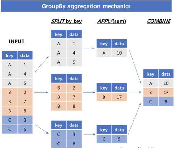
1) 그룹화(groupby)
- 같은 값을 하나로 묶어 통계 또는 집계 결과를얻기위해 사용하는 것
- 아래의 세 단계를 적용하여 데이터를 그룹화(groupping) / 특정한 col을 기준으로 데이터를 그룹핑 하여 통계에 활용하는 것
- 데이터 분할(split) : 어떠한 기준을 바탕으로 데이터를 나누는 일
- operation 적용(applying) : 각 그룹에 어떤 함수를 독립적으로 적용시키는 일
- 데이터 병합(cobine) : 적용되어 나온 결과들을 통합하는 일
- 데이터 분석에 있어 사용빈도가 높음
- groupby의 결과는 dictionary형태임
In [2]:
Image('img/groupby_agg.jpg')
Out[2]:
In [3]:
cust = pd.read_csv('data.csv')
cust
Out[3]:
base_ymdpro_tgt_perd_valcust_ctg_typecust_classsex_typeageefct_svc_countdt_stop_ynnpay_ynr3m_avg_bill_amtr3m_A_avg_arpu_amtr3m_B_avg_arpu_amtr6m_A_avg_arpu_amtr6m_B_avg_arpu_amttermination_yn01234...99259926992799289929
| 202006 | 20200630 | 10001 | C | F | 28 | 0 | N | N | 2640.0000 | 792.000000 | 1584.0000 | 0.0 | 0.0000 | Y |
| 202006 | 20200630 | 10001 | _ | _ | _ | 1 | N | N | 300.0000 | 90.000000 | 180.0000 | 0.0 | 0.0000 | Y |
| 202006 | 20200630 | 10001 | E | F | 24 | 1 | N | N | 16840.0000 | 2526.000000 | 6983.0000 | 0.0 | 6981.0000 | N |
| 202006 | 20200630 | 10001 | F | F | 32 | 1 | N | N | 15544.7334 | 2331.710010 | 6750.4666 | 0.0 | 6508.8000 | N |
| 202006 | 20200630 | 10001 | D | M | 18 | 1 | N | N | 4700.0000 | 0.000000 | 4502.0000 | 0.0 | 4507.7000 | N |
| ... | ... | ... | ... | ... | ... | ... | ... | ... | ... | ... | ... | ... | ... | ... |
| 202006 | 20200630 | 10001 | C | F | 15 | 1 | N | Y | 1296.0999 | 194.414985 | 643.1001 | 0.0 | 852.5499 | N |
| 202006 | 20200630 | 10001 | G | M | 12 | 1 | N | N | 13799.6666 | 2069.949990 | 10605.9266 | 0.0 | 10603.9266 | N |
| 202006 | 20200630 | 10005 | C | _ | _ | 1 | N | N | 1396.2000 | 1206.000000 | 0.0000 | 1212.0 | 0.0000 | N |
| 202006 | 20200630 | 10001 | C | F | 40 | 0 | N | N | 3140.0000 | 942.000000 | 1884.0000 | 0.0 | 0.0000 | Y |
| 202006 | 20200630 | 10001 | C | F | 59 | 1 | N | N | 2436.9000 | 365.535000 | 1839.9000 | 0.0 | 1919.7999 | N |
9930 rows × 15 columns
1-1) groupby의 groups 속성
- 각 그룹과 그룹에 속한 index를 dict 형태로 표현
In [4]:
# 파라미터 값으로 col의 리스트나 col을 전달
# 출력은 우선 dataframe이라고 하는 객체임(그룹을 생성까지 한 상태)

gender_group = cust.groupby('sex_type')
gender_group
Out[4]:
<pandas.core.groupby.generic.DataFrameGroupBy object at 0x7f3222035748>In [5]:
# groups를 활용하여 그룹의 속성을 살펴보기
gender_group.groups
Out[5]:
{'F': [0, 2, 3, 5, 7, 9, 12, 13, 14, 16, 17, 19, 20, 21, 24, 25, 26, 40, 41, 43, 46, 47, 49, 51, 52, 55, 65, 69, 73, 75, 77, 79, 80, 81, 82, 85, 86, 90, 91, 93, 94, 95, 101, 105, 106, 111, 112, 116, 119, 120, 121, 127, 130, 131, 134, 135, 136, 137, 138, 142, 143, 147, 148, 149, 151, 152, 155, 156, 157, 159, 163, 164, 166, 167, 169, 173, 174, 176, 177, 181, 184, 190, 191, 193, 195, 197, 205, 206, 208, 210, 211, 213, 215, 216, 218, 221, 225, 230, 234, 235, ...], 'M': [4, 6, 8, 11, 15, 18, 22, 23, 27, 28, 29, 30, 31, 32, 33, 34, 36, 37, 38, 39, 42, 44, 45, 48, 50, 53, 54, 56, 57, 58, 59, 60, 61, 63, 64, 67, 68, 70, 74, 76, 78, 84, 87, 88, 89, 96, 97, 98, 99, 100, 103, 104, 107, 108, 109, 110, 113, 115, 117, 122, 123, 124, 125, 126, 128, 132, 133, 139, 140, 141, 144, 145, 146, 150, 153, 154, 158, 160, 161, 162, 168, 170, 171, 172, 175, 178, 179, 180, 183, 185, 186, 187, 188, 189, 192, 194, 198, 199, 200, 201, ...], '_': [1, 10, 35, 62, 66, 71, 72, 83, 92, 102, 114, 118, 129, 165, 182, 196, 228, 232, 243, 288, 314, 317, 324, 393, 394, 451, 489, 496, 501, 502, 573, 611, 629, 658, 667, 669, 676, 683, 690, 701, 708, 717, 739, 751, 758, 773, 792, 816, 820, 821, 836, 851, 864, 895, 910, 935, 937, 942, 943, 946, 950, 971, 986, 991, 992, 1005, 1008, 1011, 1012, 1015, 1021, 1023, 1027, 1056, 1058, 1062, 1077, 1088, 1102, 1108, 1147, 1171, 1174, 1185, 1196, 1209, 1214, 1215, 1237, 1240, 1241, 1273, 1281, 1284, 1296, 1302, 1314, 1330, 1360, 1363, ...]}1-2) groupby 내부 함수 활용하기
- 그룹 데이터에 적용 가능한 통계 함수(NaN은 제외하여 연산)
- count : 데이터 개수
- size : 집단별 크기
- sum : 데이터의 합
- mean, std, var : 평균, 표준편차, 분산
- min, max : 최소, 최대값
In [7]:
# count() 함수 확인
gender_group.count()
Out[7]:
base_ymdpro_tgt_perd_valcust_ctg_typecust_classageefct_svc_countdt_stop_ynnpay_ynr3m_avg_bill_amtr3m_A_avg_arpu_amtr3m_B_avg_arpu_amtr6m_A_avg_arpu_amtr6m_B_avg_arpu_amttermination_ynsex_typeFM_
| 4251 | 4251 | 4251 | 4251 | 4251 | 4251 | 4251 | 4251 | 4251 | 4251 | 4251 | 4251 | 4251 | 4251 |
| 4998 | 4998 | 4998 | 4998 | 4998 | 4998 | 4998 | 4998 | 4998 | 4998 | 4998 | 4998 | 4998 | 4998 |
| 681 | 681 | 681 | 681 | 681 | 681 | 681 | 681 | 681 | 681 | 681 | 681 | 681 | 681 |
In [8]:
# mean() 함수 확인
gender_group.mean()
Out[8]:
base_ymdpro_tgt_perd_valcust_ctg_typeefct_svc_countr3m_avg_bill_amtr3m_A_avg_arpu_amtr3m_B_avg_arpu_amtr6m_A_avg_arpu_amtr6m_B_avg_arpu_amtsex_typeFM_
| 202006.0 | 20200630.0 | 10001.001882 | 1.098800 | 9580.926307 | 1570.372299 | 5283.876950 | 452.780488 | 4961.455810 |
| 202006.0 | 20200630.0 | 10001.004802 | 1.204882 | 9839.707339 | 1778.988878 | 5342.748791 | 641.426866 | 4851.027884 |
| 202006.0 | 20200630.0 | 10006.389134 | 6.462555 | 40297.790077 | 4809.827390 | 21057.412985 | 4854.788244 | 864.386867 |
In [9]:
# max()값 확인하기
gender_group.max()
Out[9]:
base_ymdpro_tgt_perd_valcust_ctg_typecust_classageefct_svc_countdt_stop_ynnpay_ynr3m_avg_bill_amtr3m_A_avg_arpu_amtr3m_B_avg_arpu_amtr6m_A_avg_arpu_amtr6m_B_avg_arpu_amttermination_ynsex_typeFM_
| 202006 | 20200630 | 10005 | _ | _ | 9 | Y | Y | 7.979563e+04 | 5.500240e+04 | 5.710153e+04 | 2.302815e+04 | 48787.2333 | Y |
| 202006 | 20200630 | 10005 | _ | _ | 14 | Y | Y | 1.447397e+05 | 1.315815e+05 | 6.583656e+04 | 2.749282e+04 | 64947.0920 | Y |
| 202006 | 20200630 | 10010 | _ | _ | 905 | Y | Y | 1.281568e+07 | 1.188998e+06 | 7.689409e+06 | 1.208498e+06 | 18796.6266 | Y |
In [13]:
# 특정 col만 보는 경우 : gender별 r3m_avg_bill_amt의 평균
gender_group.mean()[["r3m_avg_bill_amt"]]
Out[13]:
r3m_avg_bill_amtsex_typeFM_
| 9580.926307 |
| 9839.707339 |
| 40297.790077 |
1-3) 인덱스 설정(groupby) 후 데이터 추출하기
- 성별 r3m_avg_bill_amt의 평균
In [14]:
# groupby한 상태에서 가지고 오는 경우
gender_group.mean()[['r3m_avg_bill_amt']]
Out[14]:
r3m_avg_bill_amtsex_typeFM_
| 9580.926307 |
| 9839.707339 |
| 40297.790077 |
In [15]:
# groupby하기 전 원 DataFrame에서 가지고 오는 경우(결과가 같은 의미)
cust.groupby('sex_type').mean()[['r3m_avg_bill_amt']]
Out[15]:
r3m_avg_bill_amtsex_typeFM_
| 9580.926307 |
| 9839.707339 |
| 40297.790077 |
1-4) 복수 columns을 기준으로 Groupping 하기
- groupby에 column 리스트를 전달할 수 있고 복수개의 전달도 가능함
- 통계함수를 적용한 결과는 multiindex를 갖는 DataFrame
In [16]:
# cust_class 와 sex_type으로 index를 정하고 이에따른 r3m_avg_bill_amt의 평균을 구하기
cust.groupby(['cust_class', 'sex_type']).mean()[['r3m_avg_bill_amt']]
Out[16]:
r3m_avg_bill_amtcust_classsex_typeCFM_DFM_EFM_FFM_GFM_HFM_FM_
| 3804.342244 |
| 3155.385796 |
| 4719.075980 |
| 7848.842709 |
| 7774.098954 |
| 8419.764574 |
| 11257.301485 |
| 11158.736812 |
| 12208.980550 |
| 14913.105272 |
| 15013.379957 |
| 16231.437767 |
| 16538.595017 |
| 16847.160637 |
| 20180.014811 |
| 20154.938768 |
| 21052.154088 |
| 4304.582332 |
| 4728.388010 |
| 65268.733884 |
In [17]:
# 위와 동일하게 groupby한 이후에 평균 구하기
multi_group=cust.groupby(['cust_class', 'sex_type'])
multi_group.mean()[['r3m_avg_bill_amt']]
Out[17]:
r3m_avg_bill_amtcust_classsex_typeCFM_DFM_EFM_FFM_GFM_HFM_FM_
| 3804.342244 |
| 3155.385796 |
| 4719.075980 |
| 7848.842709 |
| 7774.098954 |
| 8419.764574 |
| 11257.301485 |
| 11158.736812 |
| 12208.980550 |
| 14913.105272 |
| 15013.379957 |
| 16231.437767 |
| 16538.595017 |
| 16847.160637 |
| 20180.014811 |
| 20154.938768 |
| 21052.154088 |
| 4304.582332 |
| 4728.388010 |
| 65268.733884 |
In [18]:
# INDEX는 DEPTH가 존재함 (loc을 사용하여 원하는 것만 가지고 옴)
cust.groupby(['cust_class', 'sex_type']).mean()[['r3m_avg_bill_amt']].loc[[("D","M")]]
Out[18]:
r3m_avg_bill_amtcust_classsex_typeDM
| 7774.098954 |
1-5) index를 이용한 group by
- index가 있는 경우, groupby 함수에 level 사용 가능
- level은 index의 depth를 의미하며, 가장 왼쪽부터 0부터 증가
- set_index 함수
- column 데이터를 index 레벨로 변경하는 경우 사용
- 기존의 행 인덱스를 제거하고 데이터 열 중 하나를 인덱스로 설정
- reset_index 함수
- 인덱스 초기화
- 기존의 행 인덱스를 제거하고 인덱스를 데이터 열로 추가
In [19]:
# DataFrame 다시 한번 확인 합니다.
cust.head()
Out[19]:
base_ymdpro_tgt_perd_valcust_ctg_typecust_classsex_typeageefct_svc_countdt_stop_ynnpay_ynr3m_avg_bill_amtr3m_A_avg_arpu_amtr3m_B_avg_arpu_amtr6m_A_avg_arpu_amtr6m_B_avg_arpu_amttermination_yn01234
| 202006 | 20200630 | 10001 | C | F | 28 | 0 | N | N | 2640.0000 | 792.00000 | 1584.0000 | 0.0 | 0.0 | Y |
| 202006 | 20200630 | 10001 | _ | _ | _ | 1 | N | N | 300.0000 | 90.00000 | 180.0000 | 0.0 | 0.0 | Y |
| 202006 | 20200630 | 10001 | E | F | 24 | 1 | N | N | 16840.0000 | 2526.00000 | 6983.0000 | 0.0 | 6981.0 | N |
| 202006 | 20200630 | 10001 | F | F | 32 | 1 | N | N | 15544.7334 | 2331.71001 | 6750.4666 | 0.0 | 6508.8 | N |
| 202006 | 20200630 | 10001 | D | M | 18 | 1 | N | N | 4700.0000 | 0.00000 | 4502.0000 | 0.0 | 4507.7 | N |
1-6) MultiIndex를 이용한 groupping
In [20]:
# set_index로 index셋팅(멀티도 가능)
cust.set_index(['cust_class','sex_type'])
Out[20]:
base_ymdpro_tgt_perd_valcust_ctg_typeageefct_svc_countdt_stop_ynnpay_ynr3m_avg_bill_amtr3m_A_avg_arpu_amtr3m_B_avg_arpu_amtr6m_A_avg_arpu_amtr6m_B_avg_arpu_amttermination_yncust_classsex_typeCF__EFFFDM......CFGMC_FF
| 202006 | 20200630 | 10001 | 28 | 0 | N | N | 2640.0000 | 792.000000 | 1584.0000 | 0.0 | 0.0000 | Y |
| 202006 | 20200630 | 10001 | _ | 1 | N | N | 300.0000 | 90.000000 | 180.0000 | 0.0 | 0.0000 | Y |
| 202006 | 20200630 | 10001 | 24 | 1 | N | N | 16840.0000 | 2526.000000 | 6983.0000 | 0.0 | 6981.0000 | N |
| 202006 | 20200630 | 10001 | 32 | 1 | N | N | 15544.7334 | 2331.710010 | 6750.4666 | 0.0 | 6508.8000 | N |
| 202006 | 20200630 | 10001 | 18 | 1 | N | N | 4700.0000 | 0.000000 | 4502.0000 | 0.0 | 4507.7000 | N |
| ... | ... | ... | ... | ... | ... | ... | ... | ... | ... | ... | ... | ... |
| 202006 | 20200630 | 10001 | 15 | 1 | N | Y | 1296.0999 | 194.414985 | 643.1001 | 0.0 | 852.5499 | N |
| 202006 | 20200630 | 10001 | 12 | 1 | N | N | 13799.6666 | 2069.949990 | 10605.9266 | 0.0 | 10603.9266 | N |
| 202006 | 20200630 | 10005 | _ | 1 | N | N | 1396.2000 | 1206.000000 | 0.0000 | 1212.0 | 0.0000 | N |
| 202006 | 20200630 | 10001 | 40 | 0 | N | N | 3140.0000 | 942.000000 | 1884.0000 | 0.0 | 0.0000 | Y |
| 202006 | 20200630 | 10001 | 59 | 1 | N | N | 2436.9000 | 365.535000 | 1839.9000 | 0.0 | 1919.7999 | N |
9930 rows × 13 columns
In [21]:
# reset_index활용하여 기존 DataFrame으로 변환  (set_index <-> reset_index)
cust.set_index(['cust_class','sex_type']).reset_index()
Out[21]:
cust_classsex_typebase_ymdpro_tgt_perd_valcust_ctg_typeageefct_svc_countdt_stop_ynnpay_ynr3m_avg_bill_amtr3m_A_avg_arpu_amtr3m_B_avg_arpu_amtr6m_A_avg_arpu_amtr6m_B_avg_arpu_amttermination_yn01234...99259926992799289929
| C | F | 202006 | 20200630 | 10001 | 28 | 0 | N | N | 2640.0000 | 792.000000 | 1584.0000 | 0.0 | 0.0000 | Y |
| _ | _ | 202006 | 20200630 | 10001 | _ | 1 | N | N | 300.0000 | 90.000000 | 180.0000 | 0.0 | 0.0000 | Y |
| E | F | 202006 | 20200630 | 10001 | 24 | 1 | N | N | 16840.0000 | 2526.000000 | 6983.0000 | 0.0 | 6981.0000 | N |
| F | F | 202006 | 20200630 | 10001 | 32 | 1 | N | N | 15544.7334 | 2331.710010 | 6750.4666 | 0.0 | 6508.8000 | N |
| D | M | 202006 | 20200630 | 10001 | 18 | 1 | N | N | 4700.0000 | 0.000000 | 4502.0000 | 0.0 | 4507.7000 | N |
| ... | ... | ... | ... | ... | ... | ... | ... | ... | ... | ... | ... | ... | ... | ... |
| C | F | 202006 | 20200630 | 10001 | 15 | 1 | N | Y | 1296.0999 | 194.414985 | 643.1001 | 0.0 | 852.5499 | N |
| G | M | 202006 | 20200630 | 10001 | 12 | 1 | N | N | 13799.6666 | 2069.949990 | 10605.9266 | 0.0 | 10603.9266 | N |
| C | _ | 202006 | 20200630 | 10005 | _ | 1 | N | N | 1396.2000 | 1206.000000 | 0.0000 | 1212.0 | 0.0000 | N |
| C | F | 202006 | 20200630 | 10001 | 40 | 0 | N | N | 3140.0000 | 942.000000 | 1884.0000 | 0.0 | 0.0000 | Y |
| C | F | 202006 | 20200630 | 10001 | 59 | 1 | N | N | 2436.9000 | 365.535000 | 1839.9000 | 0.0 | 1919.7999 | N |
9930 rows × 15 columns
In [ ]:
# 멀티 인덱스 셋팅 후 인덱스 기준으로 groupby하기
# 'cust_class'와 'sex_type'을 기준으로 index를 셋팅하고 index를 기준으로 groupby하고자 하는 경우
# groupby의 level은 index가 있는 경우에 사용
cust.set_index(['cust_class','sex_type']).groupby(level=[0]).mean()
In [ ]:
cust.set_index(['cust_class','sex_type']).groupby(level=[0,1]).mean()
1-7) aggregate(집계) 함수 사용하기groupby 결과에 집계함수를 적용하여 그룹별(mean, max등) 데이터 확인 가능
In [ ]:
#그룹별로 한번에 데이터를 한번에 보는 경우
cust.set_index(['cust_class','sex_type']).groupby(level=[0,1]).aggregate([np.mean, np.max])
2. pivot / pivot_table 함수 활용
2-1. pivot 은 뭘까?
- dataframe의 형태를 변경
- 여러 분류로 섞인 행 데이터를 열 데이터로 회전 시키는 것
- pivot의 사전적의미 : (축을 중심으로)회전하다, 회전시키다.
- pivot형태 : pandas.pivot(index, columns, values) 로 사용할 컴럼을 명시
In [22]:
import numpy as np
import pandas as pd
In [26]:
data = pd.DataFrame({'cust_id': ['cust_1', 'cust_1', 'cust_1', 'cust_2', 'cust_2', 'cust_2', 'cust_3', 'cust_3', 'cust_3'],
                  'prod_cd': ['p1', 'p2', 'p3', 'p1', 'p2', 'p3', 'p1', 'p2', 'p3'],
                  'grade' : ['A', 'A', 'A', 'A', 'A', 'A', 'B', 'B', 'B'],
                  'pch_amt': [30, 10, 0, 40, 15, 30, 0, 0, 10]})
data
Out[26]:
cust_idprod_cdgradepch_amt012345678
| cust_1 | p1 | A | 30 |
| cust_1 | p2 | A | 10 |
| cust_1 | p3 | A | 0 |
| cust_2 | p1 | A | 40 |
| cust_2 | p2 | A | 15 |
| cust_2 | p3 | A | 30 |
| cust_3 | p1 | B | 0 |
| cust_3 | p2 | B | 0 |
| cust_3 | p3 | B | 10 |
In [27]:
# 행(row)는 고객ID(cust_id), 열(col)은 상품코드(prod_cd), 값은 구매금액(pch_amt)을 pivot릏 활용하여 만들어보기
data.pivot(index = "cust_id", columns = "prod_cd", values = "pch_amt")
Out[27]:
prod_cdp1p2p3cust_idcust_1cust_2cust_3
| 30 | 10 | 0 |
| 40 | 15 | 30 |
| 0 | 0 | 10 |
In [ ]:
data.pivot( ??, ??, ??)
2-2. Pivot_table은 뭘까?
pivot_table형태 : pandas.pivot_table(data, index, columns, aggfunc)
In [ ]:
# pivot_table을 활용하여 위와 동일하게 만들기
data.pivot_table(index = 'cust_id', columns ='prod_cd', values ='pch_amt')
2-3. Pivot과 Pivot_table의 차이는뭘까 ?
pivot은 안되고 pivot_table만을 사용해야 하는 경우가 있음
1) index, columns가 2개 이상인 경우?
In [28]:
data.pivot(index = ['cust_id','grade'], columns ='prod_cd', values ='pch_amt')
Out[28]:
prod_cdp1p2p3cust_idgradecust_1Acust_2Acust_3B
| 30 | 10 | 0 |
| 40 | 15 | 30 |
| 0 | 0 | 10 |
In [29]:
data.pivot_table(index = ['cust_id','grade'], columns ='prod_cd', values ='pch_amt')
Out[29]:
prod_cdp1p2p3cust_idgradecust_1Acust_2Acust_3B
| 30 | 10 | 0 |
| 40 | 15 | 30 |
| 0 | 0 | 10 |
In [30]:
data.pivot(index = 'cust_id', columns =['grade','prod_cd'], values ='pch_amt')
Out[30]:
gradeABprod_cdp1p2p3p1p2p3cust_idcust_1cust_2cust_3
| 30.0 | 10.0 | 0.0 | NaN | NaN | NaN |
| 40.0 | 15.0 | 30.0 | NaN | NaN | NaN |
| NaN | NaN | NaN | 0.0 | 0.0 | 10.0 |
In [31]:
data.pivot_table(index = 'cust_id', columns =['grade','prod_cd'], values ='pch_amt')
Out[31]:
gradeABprod_cdp1p2p3p1p2p3cust_idcust_1cust_2cust_3
| 30.0 | 10.0 | 0.0 | NaN | NaN | NaN |
| 40.0 | 15.0 | 30.0 | NaN | NaN | NaN |
| NaN | NaN | NaN | 0.0 | 0.0 | 10.0 |
2) 중복 값이 있는 경우
- pivot은 중복 값이 있는 경우 valueError를 반환함
- pivot_table은 aggregation 함수를 활용하여 처리
In [32]:
data
Out[32]:
cust_idprod_cdgradepch_amt012345678
| cust_1 | p1 | A | 30 |
| cust_1 | p2 | A | 10 |
| cust_1 | p3 | A | 0 |
| cust_2 | p1 | A | 40 |
| cust_2 | p2 | A | 15 |
| cust_2 | p3 | A | 30 |
| cust_3 | p1 | B | 0 |
| cust_3 | p2 | B | 0 |
| cust_3 | p3 | B | 10 |
In [33]:
#index로 쓰인 grade가 중복이 있음
data.pivot(index='grade', columns='prod_cd', values='pch_amt')
---------------------------------------------------------------------------
ValueError                                Traceback (most recent call last)
<ipython-input-33-ea76ee2d3bda> in <module>
      1 #index로 쓰인 grade가 중복이 있음
----> 2 data.pivot(index='grade', columns='prod_cd', values='pch_amt')

/usr/local/lib/python3.6/dist-packages/pandas/core/frame.py in pivot(self, index, columns, values)
   6676         from pandas.core.reshape.pivot import pivot
   6677
-> 6678         return pivot(self, index=index, columns=columns, values=values)
   6679
   6680     _shared_docs[

/usr/local/lib/python3.6/dist-packages/pandas/core/reshape/pivot.py in pivot(data, index, columns, values)
    475         else:
    476             indexed = data._constructor_sliced(data[values]._values, index=index)
--> 477     return indexed.unstack(columns)
    478
    479

/usr/local/lib/python3.6/dist-packages/pandas/core/series.py in unstack(self, level, fill_value)
   3901         from pandas.core.reshape.reshape import unstack
   3902
-> 3903         return unstack(self, level, fill_value)
   3904
   3905     # ----------------------------------------------------------------------

/usr/local/lib/python3.6/dist-packages/pandas/core/reshape/reshape.py in unstack(obj, level, fill_value)
    423             return _unstack_extension_series(obj, level, fill_value)
    424         unstacker = _Unstacker(
--> 425             obj.index, level=level, constructor=obj._constructor_expanddim,
    426         )
    427         return unstacker.get_result(

/usr/local/lib/python3.6/dist-packages/pandas/core/reshape/reshape.py in __init__(self, index, level, constructor)
    118             raise ValueError("Unstacked DataFrame is too big, causing int32 overflow")
    119
--> 120         self._make_selectors()
    121
    122     @cache_readonly

/usr/local/lib/python3.6/dist-packages/pandas/core/reshape/reshape.py in _make_selectors(self)
    167
    168         if mask.sum() < len(self.index):
--> 169             raise ValueError("Index contains duplicate entries, cannot reshape")
    170
    171         self.group_index = comp_index

ValueError: Index contains duplicate entries, cannot reshape
In [34]:
#index로 쓰인 grade가 중복이 있음
data.pivot_table(index='grade', columns='prod_cd', values='pch_amt')
Out[34]:
prod_cdp1p2p3gradeAB
| 35.0 | 12.5 | 15.0 |
| 0.0 | 0.0 | 10.0 |
3) 집계 처리가 필요한 경우
pivot_table은 aggregation 함수를 활용하여 처리
In [35]:
# aggfunc를 sum으로 구하기 (shift+tab)
data.pivot_table(index='grade', columns='prod_cd', values='pch_amt', aggfunc=np.sum)
Out[35]:
prod_cdp1p2p3gradeAB
| 70 | 25 | 30 |
| 0 | 0 | 10 |
In [36]:
# 위와 같은결과 (shift+tab)
pd.pivot_table(data, index='grade', columns='prod_cd', values='pch_amt', aggfunc=np.sum)
Out[36]:
prod_cdp1p2p3gradeAB
| 70 | 25 | 30 |
| 0 | 0 | 10 |
In [37]:
# margins=True 옵션으로 행/열 기준의 집계도 확인 가능
pd.pivot_table(data, index='grade', columns='prod_cd', values='pch_amt', aggfunc=np.sum, margins=True)
Out[37]:
prod_cdp1p2p3AllgradeABAll
| 70 | 25 | 30 | 125 |
| 0 | 0 | 10 | 10 |
| 70 | 25 | 40 | 135 |
In [38]:
# aggfunc를 mean으로 구하기(default가 mean임)
pd.pivot_table(data, index='grade', columns='prod_cd', values='pch_amt', aggfunc=np.mean, margins=True)
Out[38]:
prod_cdp1p2p3AllgradeABAll
| 35.000000 | 12.500000 | 15.000000 | 20.833333 |
| 0.000000 | 0.000000 | 10.000000 | 3.333333 |
| 23.333333 | 8.333333 | 13.333333 | 15.000000 |
3. stack, unstack 함수 활용
In [39]:
df = pd.DataFrame({
    '지역': ['서울', '서울', '서울', '경기', '경기', '부산', '서울', '서울', '부산', '경기', '경기', '경기'],
    '요일': ['월요일', '화요일', '수요일', '월요일', '화요일', '월요일', '목요일', '금요일', '화요일', '수요일', '목요일', '금요일'],
    '강수량': [100, 80, 1000, 200, 200, 100, 50, 100, 200, 100, 50, 100],
    '강수확률': [80, 70, 90, 10, 20, 30, 50, 90, 20, 80, 50, 10]})

df
Out[39]:
지역요일강수량강수확률01234567891011
| 서울 | 월요일 | 100 | 80 |
| 서울 | 화요일 | 80 | 70 |
| 서울 | 수요일 | 1000 | 90 |
| 경기 | 월요일 | 200 | 10 |
| 경기 | 화요일 | 200 | 20 |
| 부산 | 월요일 | 100 | 30 |
| 서울 | 목요일 | 50 | 50 |
| 서울 | 금요일 | 100 | 90 |
| 부산 | 화요일 | 200 | 20 |
| 경기 | 수요일 | 100 | 80 |
| 경기 | 목요일 | 50 | 50 |
| 경기 | 금요일 | 100 | 10 |
3-1. stack & unstack
- stack : 컬럼 레벨에서 인덱스 레벨로 dataframe 변경
- 즉, 데이터를 row 레벨로 쌓아올리는 개념으로 이해하면 쉬움
- unstack : 인덱스 레벨에서 컬럼 레벨로 dataframe 변경
- stack의 반대 operation
- 둘은 역의 관계에 있음
In [40]:
# '지역'과 '요일'두개로 인덱스를 설정하고 별도의 DataFrame으로 설정 하기 - (직접 타이핑 해보세요)
new_df = df.set_index(['지역', '요일'])
new_df
Out[40]:
강수량강수확률지역요일서울월요일화요일수요일경기월요일화요일부산월요일서울목요일금요일부산화요일경기수요일목요일금요일
| 100 | 80 |
| 80 | 70 |
| 1000 | 90 |
| 200 | 10 |
| 200 | 20 |
| 100 | 30 |
| 50 | 50 |
| 100 | 90 |
| 200 | 20 |
| 100 | 80 |
| 50 | 50 |
| 100 | 10 |
In [41]:
# 첫번째 레벨의 인덱스(지역)를 컬럼으로 이동 / 인덱스도 레벨이 있음
new_df.unstack(0)
Out[41]:
강수량강수확률지역경기부산서울경기부산서울요일금요일목요일수요일월요일화요일
| 100.0 | NaN | 100.0 | 10.0 | NaN | 90.0 |
| 50.0 | NaN | 50.0 | 50.0 | NaN | 50.0 |
| 100.0 | NaN | 1000.0 | 80.0 | NaN | 90.0 |
| 200.0 | 100.0 | 100.0 | 10.0 | 30.0 | 80.0 |
| 200.0 | 200.0 | 80.0 | 20.0 | 20.0 | 70.0 |
In [42]:
# 두번째 레벨의 인덱스를 컬럼으로 이동
new_df.unstack(1)
Out[42]:
강수량강수확률요일금요일목요일수요일월요일화요일금요일목요일수요일월요일화요일지역경기부산서울
| 100.0 | 50.0 | 100.0 | 200.0 | 200.0 | 10.0 | 50.0 | 80.0 | 10.0 | 20.0 |
| NaN | NaN | NaN | 100.0 | 200.0 | NaN | NaN | NaN | 30.0 | 20.0 |
| 100.0 | 50.0 | 1000.0 | 100.0 | 80.0 | 90.0 | 50.0 | 90.0 | 80.0 | 70.0 |
In [43]:
new_df
Out[43]:
강수량강수확률지역요일서울월요일화요일수요일경기월요일화요일부산월요일서울목요일금요일부산화요일경기수요일목요일금요일
| 100 | 80 |
| 80 | 70 |
| 1000 | 90 |
| 200 | 10 |
| 200 | 20 |
| 100 | 30 |
| 50 | 50 |
| 100 | 90 |
| 200 | 20 |
| 100 | 80 |
| 50 | 50 |
| 100 | 10 |
In [44]:
# new_df.unstack(0)상태에서 첫번째 레벨의 컬럼(강수량과 강수확률)을 인덱스로 이동(stack(0))
new_df.unstack(0)
# new_df.unstack(0).stack(0)
Out[44]:
강수량강수확률지역경기부산서울경기부산서울요일금요일목요일수요일월요일화요일
| 100.0 | NaN | 100.0 | 10.0 | NaN | 90.0 |
| 50.0 | NaN | 50.0 | 50.0 | NaN | 50.0 |
| 100.0 | NaN | 1000.0 | 80.0 | NaN | 90.0 |
| 200.0 | 100.0 | 100.0 | 10.0 | 30.0 | 80.0 |
| 200.0 | 200.0 | 80.0 | 20.0 | 20.0 | 70.0 |
In [45]:
# 지역을 인덱스로 이동(stack(1))
new_df.unstack(0).stack(1)
Out[45]:
강수량강수확률요일지역금요일경기서울목요일경기서울수요일경기서울월요일경기부산서울화요일경기부산서울
| 100.0 | 10.0 |
| 100.0 | 90.0 |
| 50.0 | 50.0 |
| 50.0 | 50.0 |
| 100.0 | 80.0 |
| 1000.0 | 90.0 |
| 200.0 | 10.0 |
| 100.0 | 30.0 |
| 100.0 | 80.0 |
| 200.0 | 20.0 |
| 200.0 | 20.0 |
| 80.0 | 70.0 |
Chapter 3. DataFrame 병합하기
1. concat함수 활용
두 개 이상의 데이터프레임을 하나로 합치는 데이터 병합(merge)이나 연결(concatenate)을 지원합니다.
In [2]:
import pandas as pd
import numpy as np
1-1. concat 함수 사용하여 DataFrame 병합하기
- pandas.concat 함수 (배열결합 : concatenate)
- 데이터의 속성 형태가 동일한 데이터 셋 끼리 합칠때 사용 (DataFrame을 물리적으로 붙여주는 함수)
- 열 or 행 레벨로 병합하는 것
1) column명이 같은 경우
ignore_index, axis 활용
In [2]:
# df1, df2를 생성, 컬럼명이 같음
df1 = pd.DataFrame({'key1' : [0,1,2,3,4], 'value1' : ['a', 'b', 'c','d','e']}, index=[0,1,2,3,4])
df2 = pd.DataFrame({'key1' : [3,4,5,6,7], 'value1' : ['c','d','e','f','g']}, index=[3,4,5,6,7])
In [3]:
df1
Out[3]:
key1value101234
| 0 | a |
| 1 | b |
| 2 | c |
| 3 | d |
| 4 | e |
In [4]:
df2
Out[4]:
key1value134567
| 3 | c |
| 4 | d |
| 5 | e |
| 6 | f |
| 7 | g |
concat함수 옵션
- ignore_index : 기존 index를 무시하고자 하는 경우
- False : 기존 index유지(default) / True : 기존 index무시(index재배열)
- axis
- 0 : 위+아래로 합치기(row레벨) / 1 : 왼쪽+오른쪽으로 합치기(col레벨)
In [5]:
# ignore_index = False, True 에 대한 비교  (직접 타이핑 해보세요)
pd.concat([df1, df2], ignore_index=False)
Out[5]:
key1value10123434567
| 0 | a |
| 1 | b |
| 2 | c |
| 3 | d |
| 4 | e |
| 3 | c |
| 4 | d |
| 5 | e |
| 6 | f |
| 7 | g |
In [6]:
# axis=0, 1 에 대한 비교 (직접 타이핑 해보세요)
pd.concat([df1, df2], axis =0)
Out[6]:
key1value10123434567
| 0 | a |
| 1 | b |
| 2 | c |
| 3 | d |
| 4 | e |
| 3 | c |
| 4 | d |
| 5 | e |
| 6 | f |
| 7 | g |
2) column명이 다른 경우
- concat함수중에 join에 대한이해
- join 방식은 outer의 경우 합집합, inner의 경우 교집합을 의미
In [7]:
# 컬럼 명이 다른 데이터프레임 2개 생성
df3 = pd.DataFrame({'a':['a0','a1','a2', 'a3'], 'b':['b0','b1','b2','b3'], 'c':['c0','c1','c2','c3']}, index = [0,1,2,3])
df4 = pd.DataFrame({'a':['a2','a3','a4', 'a5'], 'b':['b2','b3','b4','b5'], 'c':['c2','c3','c4','c5'], 'd':['d1','d2','d3','d4']}, index = [2,3,4,5])
In [8]:
df3
Out[8]:
abc0123
| a0 | b0 | c0 |
| a1 | b1 | c1 |
| a2 | b2 | c2 |
| a3 | b3 | c3 |
In [9]:
df4
Out[9]:
abcd2345
| a2 | b2 | c2 | d1 |
| a3 | b3 | c3 | d2 |
| a4 | b4 | c4 | d3 |
| a5 | b5 | c5 | d4 |
In [10]:
# outer 방식 : 합집합 개념
pd.concat([df3, df4], join='outer')
Out[10]:
abcd01232345
| a0 | b0 | c0 | NaN |
| a1 | b1 | c1 | NaN |
| a2 | b2 | c2 | NaN |
| a3 | b3 | c3 | NaN |
| a2 | b2 | c2 | d1 |
| a3 | b3 | c3 | d2 |
| a4 | b4 | c4 | d3 |
| a5 | b5 | c5 | d4 |
In [ ]:
# inner 방식 : 교집합 개념
??
3) index 중복 여부 확인
- concat함수중에 verify_integrity에 대한 이해
- verify_integrity=False가 default임으로 error발생을 하지 않음
- verify_integrity=True인 경우 error 발생
In [11]:
# index 가 일부 중복되는 데이터프레임 2개를 생성
df5 = pd.DataFrame({'A':['A0','A1','A2'], 'B':['B0','B1','B2'], 'C':['C0','C1','C2'], 'D':['D0','D1','D2']}, index=['I0','I1','I2'])
df6 = pd.DataFrame({'A':['AA2','A3','A4'], 'B':['BB2','B3','B4'], 'C':['CC2','C3','C4'], 'D':['DD2','D3','D4']}, index=['I2','I3','I4'])
In [12]:
df5
Out[12]:
ABCDI0I1I2
| A0 | B0 | C0 | D0 |
| A1 | B1 | C1 | D1 |
| A2 | B2 | C2 | D2 |
In [13]:
df6
Out[13]:
ABCDI2I3I4
| AA2 | BB2 | CC2 | DD2 |
| A3 | B3 | C3 | D3 |
| A4 | B4 | C4 | D4 |
In [14]:
# 중복된 index를 확인할지 여부를 결정하는 파라미터 verify_integrity (기본:false)
pd.concat([df5, df6], verify_integrity=False)
Out[14]:
ABCDI0I1I2I2I3I4
| A0 | B0 | C0 | D0 |
| A1 | B1 | C1 | D1 |
| A2 | B2 | C2 | D2 |
| AA2 | BB2 | CC2 | DD2 |
| A3 | B3 | C3 | D3 |
| A4 | B4 | C4 | D4 |
In [16]:
# True 로 작성하면, index 중복이 있는 경우 error가 남
pd.concat([df5, df6], verify_integrity=True)
---------------------------------------------------------------------------
ValueError                                Traceback (most recent call last)
<ipython-input-16-dd6f199cbf94> in <module>
      1 # True 로 작성하면, index 중복이 있는 경우 error가 남
----> 2 pd.concat([df5, df6], verify_integrity=True)

/usr/local/lib/python3.6/dist-packages/pandas/core/reshape/concat.py in concat(objs, axis, join, ignore_index, keys, levels, names, verify_integrity, sort, copy)
    282         verify_integrity=verify_integrity,
    283         copy=copy,
--> 284         sort=sort,
    285     )
    286

/usr/local/lib/python3.6/dist-packages/pandas/core/reshape/concat.py in __init__(self, objs, axis, join, keys, levels, names, ignore_index, verify_integrity, copy, sort)
    452         self.copy = copy
    453
--> 454         self.new_axes = self._get_new_axes()
    455
    456     def get_result(self):

/usr/local/lib/python3.6/dist-packages/pandas/core/reshape/concat.py in _get_new_axes(self)
    519         return [
    520             self._get_concat_axis() if i == self.bm_axis else self._get_comb_axis(i)
--> 521             for i in range(ndim)
    522         ]
    523

/usr/local/lib/python3.6/dist-packages/pandas/core/reshape/concat.py in <listcomp>(.0)
    519         return [
    520             self._get_concat_axis() if i == self.bm_axis else self._get_comb_axis(i)
--> 521             for i in range(ndim)
    522         ]
    523

/usr/local/lib/python3.6/dist-packages/pandas/core/reshape/concat.py in _get_concat_axis(self)
    578             )
    579
--> 580         self._maybe_check_integrity(concat_axis)
    581
    582         return concat_axis

/usr/local/lib/python3.6/dist-packages/pandas/core/reshape/concat.py in _maybe_check_integrity(self, concat_index)
    586             if not concat_index.is_unique:
    587                 overlap = concat_index[concat_index.duplicated()].unique()
--> 588                 raise ValueError(f"Indexes have overlapping values: {overlap}")
    589
    590

ValueError: Indexes have overlapping values: Index(['I2'], dtype='object')
2. merge & join 함수 활용
2-1. DataFrame merge
- Database의 Table들을 Merge/Join하는 것과 유사함
- 특정한 column(key)을 기준으로 병합
- join 방식: how 파라미터를 통해 명시(특정한 col을 바탕으로 join 하는 것)
- inner: 기본 merge방법, 일치하는 값이 있는 경우 (Merge할 테이블의 데이터가 모두 있는 경우만 가지고 옴)
- left: left outer join (왼쪽을 기준으로 오른쪽을 채움 - 오른쪽에 데이터 없으면 NaN)
- right: right outer join
- outer: full outer join (Left와 Right를 합한 것)
In [5]:
customer = pd.DataFrame({'cust_id' : np.arange(6),
                    'name' : ['철수', '영희', '길동', '영수', '수민', '동건'],
                    '나이' : [40, 20, 21, 30, 31, 18]})

orders = pd.DataFrame({'cust_id' : [1, 1, 2, 2, 2, 3, 3, 1, 4, 9],
                    'item' : ['치약', '칫솔', '이어폰', '헤드셋', '수건', '생수', '수건', '치약', '생수', '케이스'],
                    'quantity' : [1, 2, 1, 1, 3, 2, 2, 3, 2, 1]})
In [6]:
customer
Out[6]:
cust_idname나이012345
| 0 | 철수 | 40 |
| 1 | 영희 | 20 |
| 2 | 길동 | 21 |
| 3 | 영수 | 30 |
| 4 | 수민 | 31 |
| 5 | 동건 | 18 |
In [7]:
orders
Out[7]:
cust_iditemquantity0123456789
| 1 | 치약 | 1 |
| 1 | 칫솔 | 2 |
| 2 | 이어폰 | 1 |
| 2 | 헤드셋 | 1 |
| 2 | 수건 | 3 |
| 3 | 생수 | 2 |
| 3 | 수건 | 2 |
| 1 | 치약 | 3 |
| 4 | 생수 | 2 |
| 9 | 케이스 | 1 |
1) merge함수의 on 옵션
- on : join 대상이 되는 column 명시
In [8]:
# 기본적인 Merge방식은 inner임 (직접 타이핑 해보세요)
# customer의 cust_id 0,5번과 orders의 cust_id 9번이 없는 것을 확인
pd.merge(customer, orders, on='cust_id')
Out[8]:
cust_idname나이itemquantity012345678
| 1 | 영희 | 20 | 치약 | 1 |
| 1 | 영희 | 20 | 칫솔 | 2 |
| 1 | 영희 | 20 | 치약 | 3 |
| 2 | 길동 | 21 | 이어폰 | 1 |
| 2 | 길동 | 21 | 헤드셋 | 1 |
| 2 | 길동 | 21 | 수건 | 3 |
| 3 | 영수 | 30 | 생수 | 2 |
| 3 | 영수 | 30 | 수건 | 2 |
| 4 | 수민 | 31 | 생수 | 2 |
In [9]:
# merge하고자 하는 컬럼 명칭을 on에 명시한다.
# 여러개인 경우 리스트  일치하는 것만 가지고 옴
pd.merge(customer, orders, on='cust_id', how='inner')
Out[9]:
cust_idname나이itemquantity012345678
| 1 | 영희 | 20 | 치약 | 1 |
| 1 | 영희 | 20 | 칫솔 | 2 |
| 1 | 영희 | 20 | 치약 | 3 |
| 2 | 길동 | 21 | 이어폰 | 1 |
| 2 | 길동 | 21 | 헤드셋 | 1 |
| 2 | 길동 | 21 | 수건 | 3 |
| 3 | 영수 | 30 | 생수 | 2 |
| 3 | 영수 | 30 | 수건 | 2 |
| 4 | 수민 | 31 | 생수 | 2 |
In [10]:
# 왼쪽 테이블을 기준으로 Merge (여기서는 customer기준)
# cust_id 5번이 나타났다.
pd.merge(customer, orders, on='cust_id', how='left')
Out[10]:
cust_idname나이itemquantity012345678910
| 0 | 철수 | 40 | NaN | NaN |
| 1 | 영희 | 20 | 치약 | 1.0 |
| 1 | 영희 | 20 | 칫솔 | 2.0 |
| 1 | 영희 | 20 | 치약 | 3.0 |
| 2 | 길동 | 21 | 이어폰 | 1.0 |
| 2 | 길동 | 21 | 헤드셋 | 1.0 |
| 2 | 길동 | 21 | 수건 | 3.0 |
| 3 | 영수 | 30 | 생수 | 2.0 |
| 3 | 영수 | 30 | 수건 | 2.0 |
| 4 | 수민 | 31 | 생수 | 2.0 |
| 5 | 동건 | 18 | NaN | NaN |
In [11]:
# 오른쪽 테이블을 기준으로 Merge (여기서는 orders기준)
# cust_id 9번이 나타났다.
pd.merge(customer, orders, on='cust_id', how='left')
Out[11]:
cust_idname나이itemquantity012345678910
| 0 | 철수 | 40 | NaN | NaN |
| 1 | 영희 | 20 | 치약 | 1.0 |
| 1 | 영희 | 20 | 칫솔 | 2.0 |
| 1 | 영희 | 20 | 치약 | 3.0 |
| 2 | 길동 | 21 | 이어폰 | 1.0 |
| 2 | 길동 | 21 | 헤드셋 | 1.0 |
| 2 | 길동 | 21 | 수건 | 3.0 |
| 3 | 영수 | 30 | 생수 | 2.0 |
| 3 | 영수 | 30 | 수건 | 2.0 |
| 4 | 수민 | 31 | 생수 | 2.0 |
| 5 | 동건 | 18 | NaN | NaN |
In [12]:
# outer : Left와 Right를 합친 것 (합집합)
# 모든 cust_id 가 나타났다.
??
IPython -- An enhanced Interactive Python
=========================================

IPython offers a fully compatible replacement for the standard Python
interpreter, with convenient shell features, special commands, command
history mechanism and output results caching.

At your system command line, type 'ipython -h' to see the command line
options available. This document only describes interactive features.

GETTING HELP
------------

Within IPython you have various way to access help:

  ?         -> Introduction and overview of IPython's features (this screen).
  object?   -> Details about 'object'.
  object??  -> More detailed, verbose information about 'object'.
  %quickref -> Quick reference of all IPython specific syntax and magics.
  help      -> Access Python's own help system.

If you are in terminal IPython you can quit this screen by pressing `q`.


MAIN FEATURES
-------------

* Access to the standard Python help with object docstrings and the Python
  manuals. Simply type 'help' (no quotes) to invoke it.

* Magic commands: type %magic for information on the magic subsystem.

* System command aliases, via the %alias command or the configuration file(s).

* Dynamic object information:

  Typing ?word or word? prints detailed information about an object. Certain
  long strings (code, etc.) get snipped in the center for brevity.

  Typing ??word or word?? gives access to the full information without
  snipping long strings. Strings that are longer than the screen are printed
  through the less pager.

  The ?/?? system gives access to the full source code for any object (if
  available), shows function prototypes and other useful information.

  If you just want to see an object's docstring, type '%pdoc object' (without
  quotes, and without % if you have automagic on).

* Tab completion in the local namespace:

  At any time, hitting tab will complete any available python commands or
  variable names, and show you a list of the possible completions if there's
  no unambiguous one. It will also complete filenames in the current directory.

* Search previous command history in multiple ways:

  - Start typing, and then use arrow keys up/down or (Ctrl-p/Ctrl-n) to search
    through the history items that match what you've typed so far.

  - Hit Ctrl-r: opens a search prompt. Begin typing and the system searches
    your history for lines that match what you've typed so far, completing as
    much as it can.

  - %hist: search history by index.

* Persistent command history across sessions.

* Logging of input with the ability to save and restore a working session.

* System shell with !. Typing !ls will run 'ls' in the current directory.

* The reload command does a 'deep' reload of a module: changes made to the
  module since you imported will actually be available without having to exit.

* Verbose and colored exception traceback printouts. See the magic xmode and
  xcolor functions for details (just type %magic).

* Input caching system:

  IPython offers numbered prompts (In/Out) with input and output caching. All
  input is saved and can be retrieved as variables (besides the usual arrow
  key recall).

  The following GLOBAL variables always exist (so don't overwrite them!):
  _i: stores previous input.
  _ii: next previous.
  _iii: next-next previous.
  _ih : a list of all input _ih[n] is the input from line n.

  Additionally, global variables named _i<n> are dynamically created (<n>
  being the prompt counter), such that _i<n> == _ih[<n>]

  For example, what you typed at prompt 14 is available as _i14 and _ih[14].

  You can create macros which contain multiple input lines from this history,
  for later re-execution, with the %macro function.

  The history function %hist allows you to see any part of your input history
  by printing a range of the _i variables. Note that inputs which contain
  magic functions (%) appear in the history with a prepended comment. This is
  because they aren't really valid Python code, so you can't exec them.

* Output caching system:

  For output that is returned from actions, a system similar to the input
  cache exists but using _ instead of _i. Only actions that produce a result
  (NOT assignments, for example) are cached. If you are familiar with
  Mathematica, IPython's _ variables behave exactly like Mathematica's %
  variables.

  The following GLOBAL variables always exist (so don't overwrite them!):
  _ (one underscore): previous output.
  __ (two underscores): next previous.
  ___ (three underscores): next-next previous.

  Global variables named _<n> are dynamically created (<n> being the prompt
  counter), such that the result of output <n> is always available as _<n>.

  Finally, a global dictionary named _oh exists with entries for all lines
  which generated output.

* Directory history:

  Your history of visited directories is kept in the global list _dh, and the
  magic %cd command can be used to go to any entry in that list.

* Auto-parentheses and auto-quotes (adapted from Nathan Gray's LazyPython)

  1. Auto-parentheses

     Callable objects (i.e. functions, methods, etc) can be invoked like
     this (notice the commas between the arguments)::

         In [1]: callable_ob arg1, arg2, arg3

     and the input will be translated to this::

         callable_ob(arg1, arg2, arg3)

     This feature is off by default (in rare cases it can produce
     undesirable side-effects), but you can activate it at the command-line
     by starting IPython with `--autocall 1`, set it permanently in your
     configuration file, or turn on at runtime with `%autocall 1`.

     You can force auto-parentheses by using '/' as the first character
     of a line.  For example::

          In [1]: /globals             # becomes 'globals()'

     Note that the '/' MUST be the first character on the line!  This
     won't work::

          In [2]: print /globals    # syntax error

     In most cases the automatic algorithm should work, so you should
     rarely need to explicitly invoke /. One notable exception is if you
     are trying to call a function with a list of tuples as arguments (the
     parenthesis will confuse IPython)::

          In [1]: zip (1,2,3),(4,5,6)  # won't work

     but this will work::

          In [2]: /zip (1,2,3),(4,5,6)
          ------> zip ((1,2,3),(4,5,6))
          Out[2]= [(1, 4), (2, 5), (3, 6)]

     IPython tells you that it has altered your command line by
     displaying the new command line preceded by -->.  e.g.::

          In [18]: callable list
          -------> callable (list)

  2. Auto-Quoting

     You can force auto-quoting of a function's arguments by using ',' as
     the first character of a line.  For example::

          In [1]: ,my_function /home/me   # becomes my_function("/home/me")

     If you use ';' instead, the whole argument is quoted as a single
     string (while ',' splits on whitespace)::

          In [2]: ,my_function a b c   # becomes my_function("a","b","c")
          In [3]: ;my_function a b c   # becomes my_function("a b c")

     Note that the ',' MUST be the first character on the line!  This
     won't work::

          In [4]: x = ,my_function /home/me    # syntax error
2) index 기준으로 join하기
In [13]:
#cust_id를 기준으로 인덱스 생성하기 (set_index활용)  (직접 타이핑 해보세요)
cust1 = customer.set_index('cust_id')
order1 = orders.set_index('cust_id')
In [14]:
cust1
Out[14]:
name나이cust_id012345
| 철수 | 40 |
| 영희 | 20 |
| 길동 | 21 |
| 영수 | 30 |
| 수민 | 31 |
| 동건 | 18 |
In [15]:
order1
Out[15]:
itemquantitycust_id1122233149
| 치약 | 1 |
| 칫솔 | 2 |
| 이어폰 | 1 |
| 헤드셋 | 1 |
| 수건 | 3 |
| 생수 | 2 |
| 수건 | 2 |
| 치약 | 3 |
| 생수 | 2 |
| 케이스 | 1 |
In [16]:
# on을 명시할 필요 없이 index를 merge 하고자 하는 경우
pd.merge(cust1, order1, left_index=True, right_index=True).reset_index()
#inner와 동일한 형태
Out[16]:
cust_idname나이itemquantity012345678
| 1 | 영희 | 20 | 치약 | 1 |
| 1 | 영희 | 20 | 칫솔 | 2 |
| 1 | 영희 | 20 | 치약 | 3 |
| 2 | 길동 | 21 | 이어폰 | 1 |
| 2 | 길동 | 21 | 헤드셋 | 1 |
| 2 | 길동 | 21 | 수건 | 3 |
| 3 | 영수 | 30 | 생수 | 2 |
| 3 | 영수 | 30 | 수건 | 2 |
| 4 | 수민 | 31 | 생수 | 2 |
연습문제1) 가장 많이 팔린 아이템은?
- Hint : merge, groupby, sum, sort_values 활용
- 아이템이 중요함으로 orders DF이 중요
-
- customer, orders 를 merge함. how는?
-
- groupby이용하여 item을 grouping후 sum
-
- sort_values를 이용하여 'quantity'를 기준으로 '내림차순'으로 정렬
In [17]:
pd.merge(customer, orders, on='cust_id', how='right').groupby('item').sum().sort_values(by='quantity', ascending=True)
Out[17]:
cust_id나이quantityitem이어폰케이스헤드셋칫솔생수치약수건
| 2 | 21.0 | 1 |
| 9 | 0.0 | 1 |
| 2 | 21.0 | 1 |
| 1 | 20.0 | 2 |
| 7 | 61.0 | 4 |
| 2 | 40.0 | 4 |
| 5 | 51.0 | 5 |
연습문제2) 영희가 가장 많이 구매한 아이템은?
-
- 우선 사람과 아이템 별로 sum을 해서(groupby시 "이름"과 "아이템"기준으로 합을 구하고)
-
- loc을 활용하여 (영희의 row의 quantity만 확인)
In [18]:
pd.merge(customer, orders, on="cust_id", how="inner").groupby(["name","item"]).sum()
Out[18]:
cust_id나이quantitynameitem길동수건이어폰헤드셋수민생수영수생수수건영희치약칫솔
| 2 | 21 | 3 |
| 2 | 21 | 1 |
| 2 | 21 | 1 |
| 4 | 31 | 2 |
| 3 | 30 | 2 |
| 3 | 30 | 2 |
| 2 | 40 | 4 |
| 1 | 20 | 2 |
2-2. join 함수
- index가 있는 경우 사용(행 인덱스를 기준으로 결합)
- 내부적으로 pandas.merge 함수를 기반으로 만들어짐
- 기본적으로 index를 사용하여 left join
- 형태 : Dataframe1.join(Dataframe2. how='left')
In [19]:
cust1.join(order1, how='inner')
Out[19]:
name나이itemquantitycust_id111222334
| 영희 | 20 | 치약 | 1 |
| 영희 | 20 | 칫솔 | 2 |
| 영희 | 20 | 치약 | 3 |
| 길동 | 21 | 이어폰 | 1 |
| 길동 | 21 | 헤드셋 | 1 |
| 길동 | 21 | 수건 | 3 |
| 영수 | 30 | 생수 | 2 |
| 영수 | 30 | 수건 | 2 |
| 수민 | 31 | 생수 | 2 |
'경기도 인공지능 개발 과정 > Python' 카테고리의 다른 글
| [Python] AutoEncoder를 활용한 image-search-engine (이미지 유사도 검증) (0) | 2022.09.10 |
|---|---|
| [AIFB] matplolib, seaborn 시각화 (0) | 2022.08.08 |
| [Python] Image segmentation 실습 (1) | 2022.08.04 |
| [Python] Simple YoLo 실습 (2) | 2022.08.04 |
| [python] 텐서플로 object_detection 실습 (2) | 2022.08.04 |